This is a web version of our ICLR paper Learning is Forgetting: LLM Training As Lossy Compression. A less technical companion piece is available here
1 Introduction
We still have a limited understanding of how Large Language Models (LLMs) achieve impressive results across a wide array of tasks (Devlin et al. 2019; Grattafiori et al. 2024). While a growing body of work interprets LLMs using behavioural experiments, probing, or causal interventions, the scale of these models makes understanding how their representation spaces are structured a continued challenge. Here we look at an LLM as an instance of lossy compression, offering an account of how models represent information during training and what information matters for performance.
Lossy compression represents data efficiently by preserving only the information from a source relevant to a goal. While uncompressed audio recordings intended for human listeners can be gigabytes in size, MP3 files save space by discarding frequencies typically outside the range of human hearing (Jayant, Johnston, and Safranek 1993); similarly, a JPEG file omits subtle colour variations that are difficult for the human eye to perceive. We draw a parallel with LLMs, which are expected to generate responses humans prefer, after being trained on trillions of tokens — more language data than a human hears in 200 lifetimes. More generally, compression is thought to underpin learning in both humans and models (Feldman 2016), and giving a formal account of LLM pre-training in terms of compression allows us to work towards a unified theory of representation learning. We present results showing that over the course of pre-training LLMs optimally compress the information present in their training data for next sequence prediction.
Compression is inherently opinionated — some information from the source is preserved, some is forgotten to save space. Information Theory (Shannon 1948) provides a formal framework to describe this process, letting us both quantify the information present in a representation and compute a bound where it is optimally compressed with respect to the data it represents. Our results build on the Information Bottleneck (IB) theory of deep learning (Tishby and Zaslavsky 2015), showing pre-training follows a two phase trajectory: first increasing mutual information with the training objective, before compressing input information. Across a wide array of LLMs we find each model compresses differently, with the optimality of a model’s compression and the information it preserves predicting performance on downstream benchmarks.
A hallmark of large-scale distributed systems, like neural networks, is that they are difficult to understand as a function of their parts alone (Anderson 1972; Mitchell 2009). Our approach to interpretability allows us to consider learning and generalisation at the scale of an entire model, rather than studying individual circuits, heads, or neurons within it. Additionally, it allows us to frame how models do so well at so much in terms of existing theories of learning and compression, while providing actionable insights at LLM scale.
In what follows we focus on offering concrete answers to three questions: Do LLMs optimally compress their representations? What information survives that compression? What representational structures drive performance? In summary, our core findings are:
- Pre-training dynamics for LLMs closely follow theoretical predictions from the Information Bottleneck, with models first expanding representations before slowly approaching optimal compression.
- Scale conditions these dynamics, with smaller models (below 7 billion parameters) struggling to achieve meaningful compression later in training.
- How optimally compressed a model is correlates significantly with performance across six benchmarks for six families of open-weights large language models, letting us directly relate representation structure to behaviour.
- By quantifying the amount of preference information in a model we get a quantification of how aligned representations are with preference distinctions, which significantly predicts downstream performance across 47 LLMs (\(r=0.76, p<0.001\)).
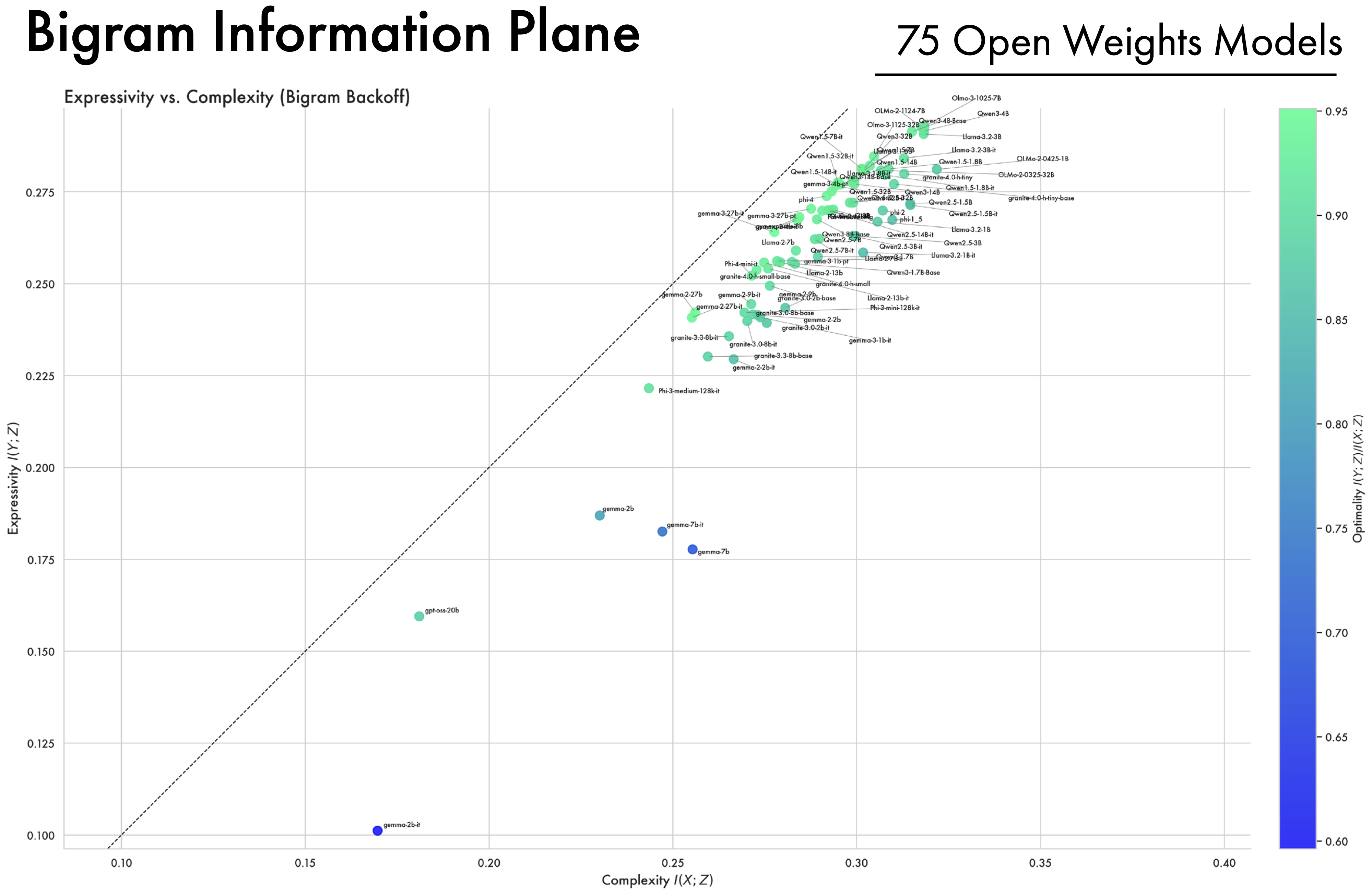
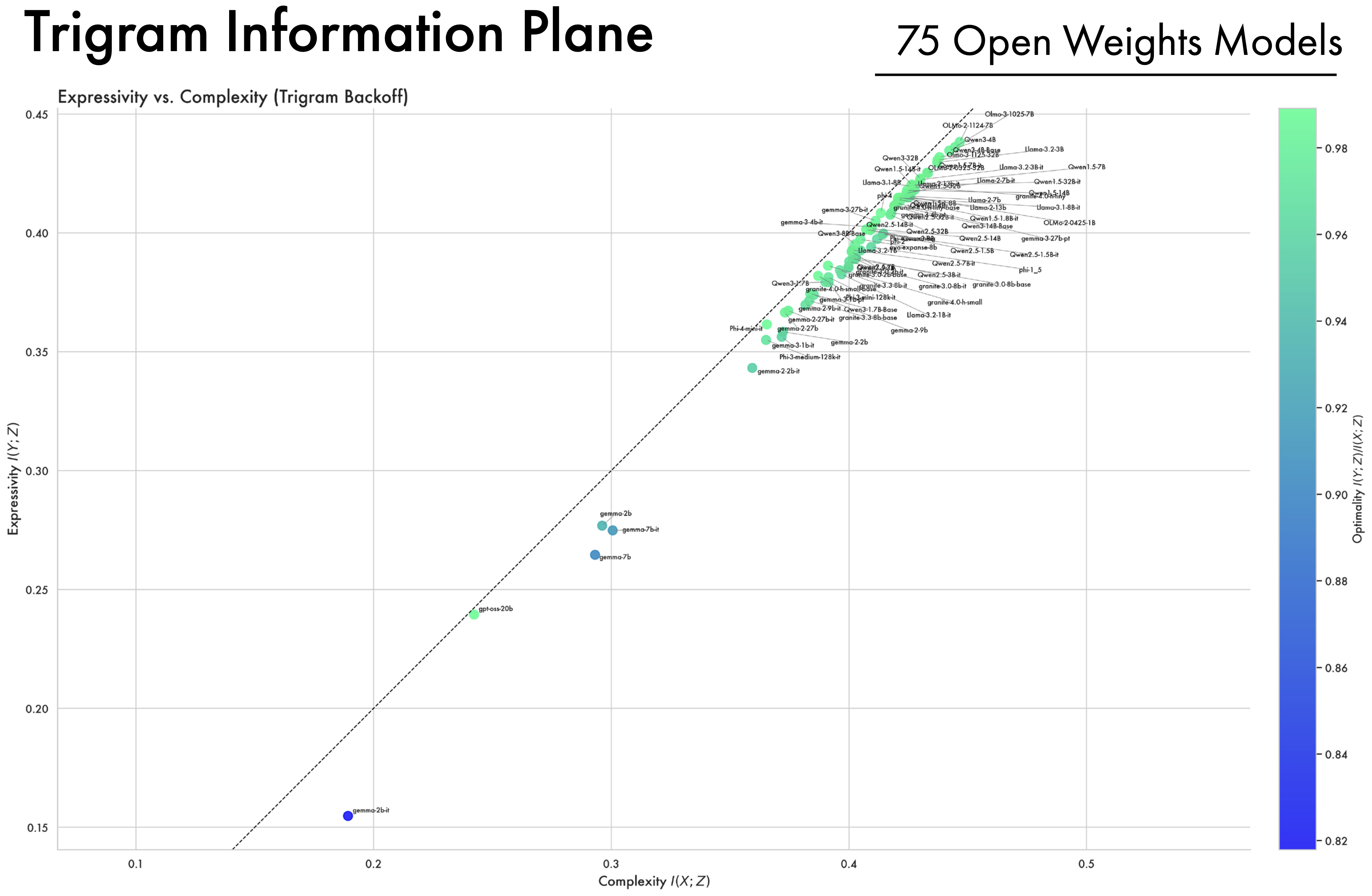
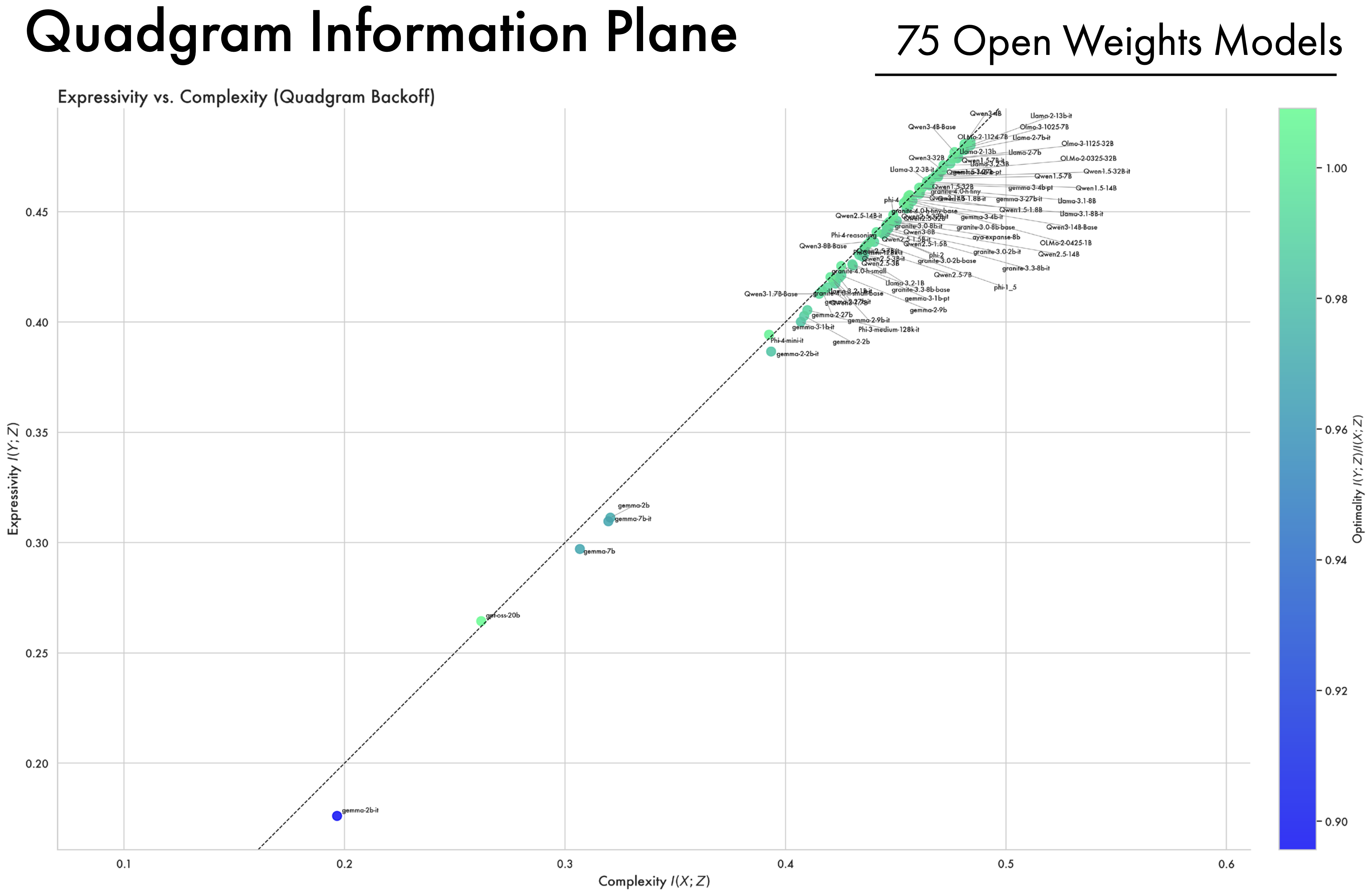
- Finally, we compare a wide array of open-weight models across 5 model families, showing they all converge near optimal compression.
3 Methods
3.1 Entropy Estimation
Let \(T \in \mathbb{Z}^{B\times S}\) be a batch of \(B\) tokenized samples with sequence length \(S\), drawn from a corpus of text data \(\mathcal{T}\), and let \(\theta\) be a model with \(L\) layers and representation dimension \(h\); the corresponding encoded representations are \(Z \in \mathbb{R}^{L \times B \times S \times h}\). Let \(X\in \mathbb{Z}^{B\times S}\) be feature labels for the text in \(T\). For example, when we look at optimal compression with respect to the IB bound, these labels \(X\) are the token ids for the model inputs; however, when analysing representation information more generally, these can be other input features, such as preference label or language ID. It is desirable to compute the mutual information \(I(X;Z)\) using Shannon entropy as opposed to differential entropy. Previous work quantises \(Z\) into \(n\) bins, to get a discrete encoding \(\hat{Z}\) (Voita, Sennrich, and Titov 2019; Shwartz-Ziv and Tishby 2017). Unfortunately these approaches have memory and resource requirements that make them difficult to apply at LLM scale.2
2 For discussion of Shannon entropy and why previous approaches are not scalable see Appendix E.6 and E.7.
As a result we use the soft-entropy estimator from Conklin (2025) — an efficient differentiable relaxation of a binning-based estimate that has been shown to converge to the true entropy of a distribution. This estimator is not original to our work, but we are the first to apply it to analyse LLMs using rate distortion theory.
We first compute \(\bar{Z}\), the normalization of \(Z\) to lie on the surface of the unit sphere \(\mathbb{S}^h\) in \(\mathbb{R}^h\). Then we compute \(W\) by sampling \(n\) points \(\{w_i\}_{i=1}^n\) uniformly at random from \(\mathbb{S}^h\).3 For each normalized representation \(\bar{z} \in \mathbb{R}^h\), we compute a vector whose \(i^{th}\) entry is the cosine between \(\bar{z}\) and \(w_i\), then apply softmax to that vector — softly assigning each embedding \(\bar{z}\) to the points in \(W\). More formally, each \((l,b,s) \in [L] \times [B] \times [S]\) tensor \(\bar{Z}\) (whose shape coincides with \(Z\)) is defined so that \(\bar{Z}_{l,b,s, :} = Z_{l,b,s, :} / \| Z_{l,b,s, :} \|\), and we stack the uniform samples \(\{ w_i\}_{i=1}^n\) into a matrix \(W \in \mathbb{R}^{h \times n}\). The soft-quantisation of \(Z\) is then given by \(\check{Z} \in \mathbb{R}^{L \times B \times S \times n}\) for \((l,b,s) \in [L] \times [B] \times [S]\):
3 This is equivalent to sampling from an isometric \(h\)-dimensional multivariate normal, \(\tilde{w}_i \sim \mathcal{N}(0, Id_h)\), and scaling to unit length, \(w_i = \frac{\tilde{w}_i}{||\tilde{w}_i||}\).
\[ \{w_i\}_{i=1}^n \sim \text{Unif}(\mathbb{S}^h), \qquad W_{:, i} = w_i, \qquad \check{Z}_{l, b, s, :} = \mathrm{softmax}\!\Big(\frac{\sum_{j=1}^h \bar{Z}_{l,b,s,j} W_{j,:}}{\epsilon}\Big) \]
where \(\epsilon\) is a temperature parameter, which we set to enable direct comparison of representations with different dimensionalities following the calibration procedure described in Appendix E.1. Each vector \(\check{Z}_{l, b, s,:}\) is a probability vector. Let \(\hat{Z} \in \mathbb{R}^{L \times n}\) be the matrix obtained from tensor \(\check{Z}\) by averaging over the batch and sequence dimensions, and let \(\hat{z}_l\) be the \(l\)-th row of this matrix:
\[ \hat{Z} = \frac{1}{BS} \sum_{b=1}^B \sum_{s=1}^S \check{Z}_{:,b,s,:}, \qquad \hat{z}_l = \hat{Z}_{l, :}, \quad H(\hat{z}_l) = - \sum_{j=1}^n \hat{z}_{l, j} \log \hat{z}_{l,j} \]
Vectors \(\hat{z}_l\) are probability vectors for each layer \(l \in [L]\) describing a categorical distribution over \(n\) categories, so we can compute the Shannon entropy \(H(\hat{z}_l)\) as above.
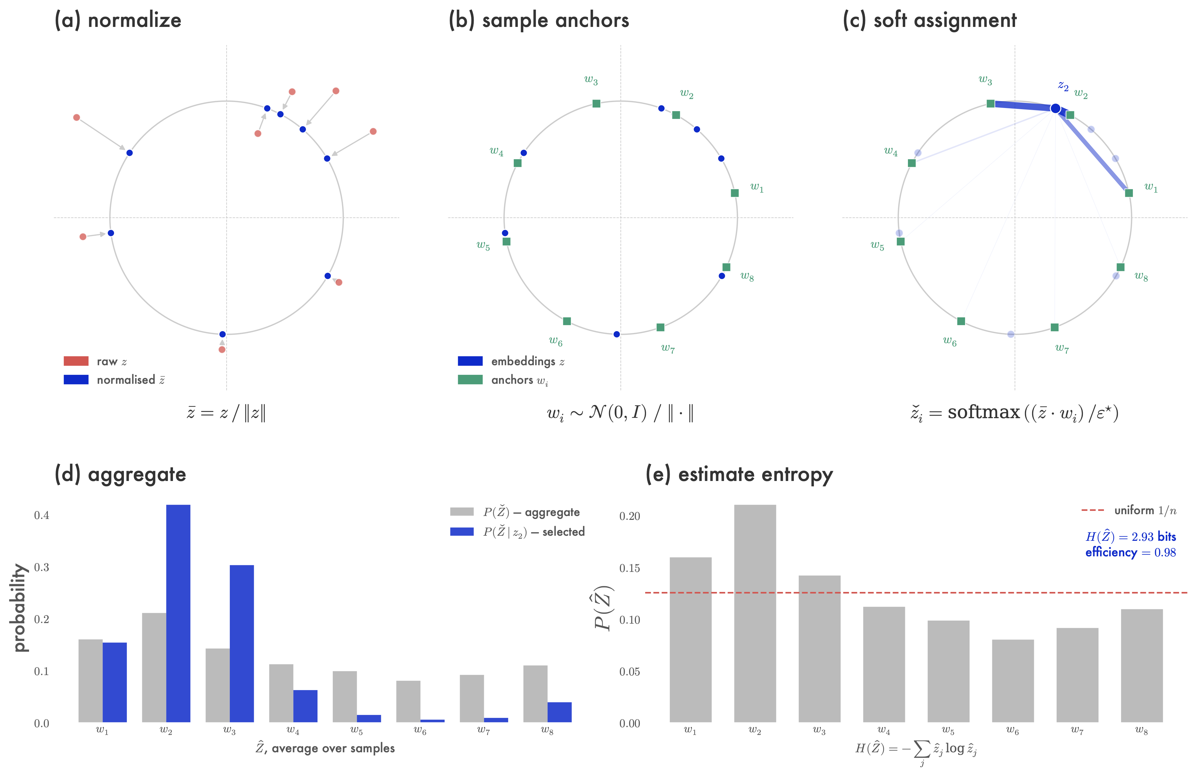
Due to the normalisation step during quantisation, this distribution intuitively estimates the probability that a representation in a layer \(l\) lies along a particular angle with respect to the origin. To estimate the entropy in an entire model, denoted \(H(Z)\), we average entropy across layers. Efficiency (Wilcox 1967) normalises \(H\) by the entropy of a uniform distribution \(\log(n)\), thereby bounding the entropic quantity between 0 and 1. To aid interpretability we convert \(H(Z)\) to an efficiency \(\mathcal{H}(Z)\) by normalising by the entropy of a uniform distribution at each layer. These definitions can also be conditioned on the feature labels \(X\):
\[ \mathcal{H}(Z) := \frac{1}{L\log(n)}\sum_{l=1}^{L} H(\hat{z}_l), \qquad \mathcal{H}(Z| X=x) := \frac{1}{L \log (n)} \sum_{l=1}^L H(\hat{z}_l | X=x) \]
This now allows us to efficiently compute the mutual information between input features \(X\) and encodings across an entire model, regardless of model size:
\[ I(X; Z) := \mathcal{H}(Z) - \sum_{x \in X} P(X=x)\,\mathcal{H}(Z| X=x) \]
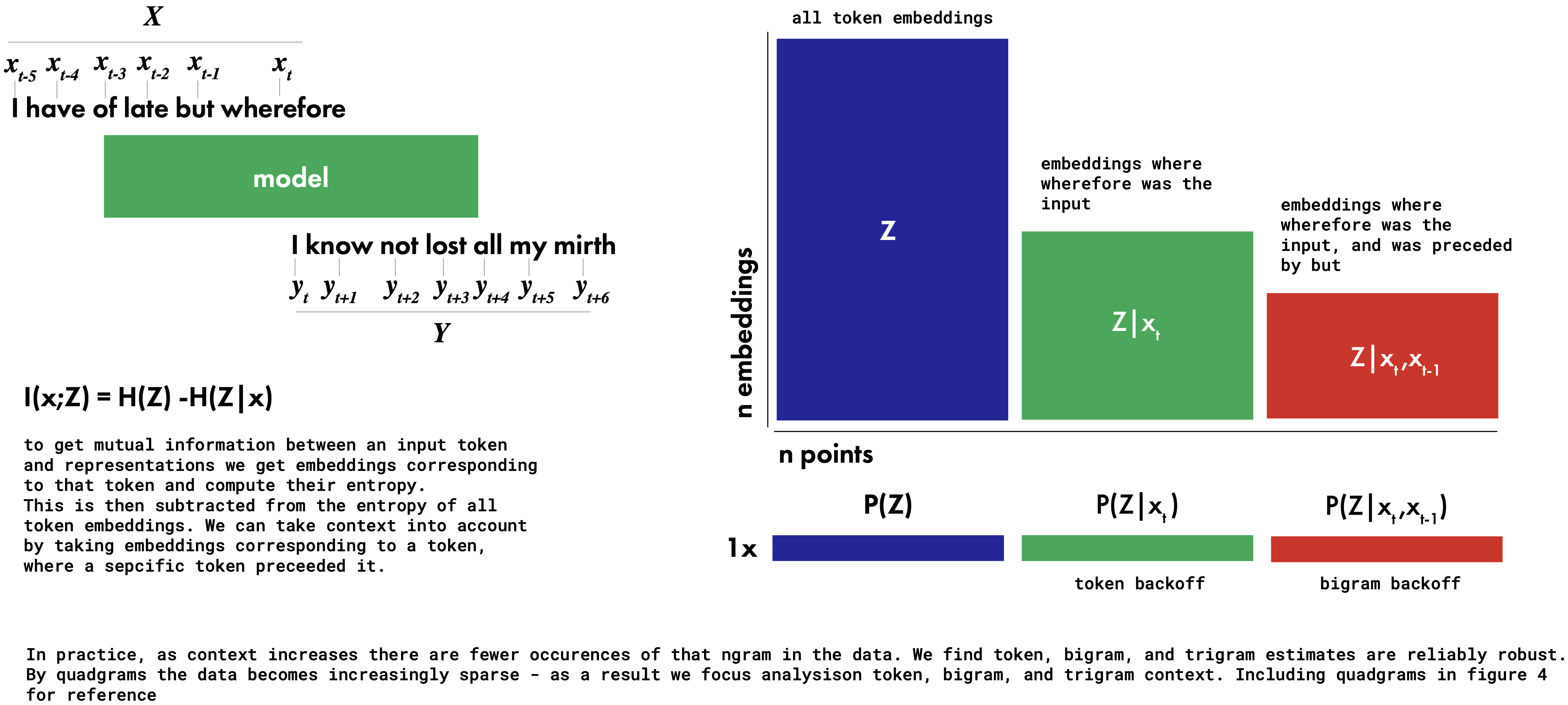
3.2 Mutual Informations & Back-off
To determine whether or not a model is optimally compressed with respect to some data we need to compute mutual informations with respect to input and output labels. LLMs are trained with inputs as preceding context and outputs as trailing context. Maintaining conditional estimates of a token embedding given a preceding context \(P(Z|X)\) for every possible context window proves intractable, and many contexts occur only once in the training data. Accordingly, like many other works on language modelling, we approximate the distribution over possible sequences using n-grams with a kind of back-off (Katz 1987). By conditioning on finite widths of preceding context we can tractably approximate \(P(Z|X)\); the maximum width we consider here are quad-grams, by which point \(I(X;Z)\) begins to converge. By backing off further (e.g. to trigrams, bigrams, and tokens) we can also estimate how much different context widths contribute to information in a model. We vary the degree of backoff equally for both the input \(P(Z|X)\) and output \(P(Z|Y)\) distributions, because during training a model receives gradient information from the full trailing context \(Y\) due to teacher forcing.
In comparing different models we would like to be able to determine how close a given representation system is to the IB bound — by extension, how optimally compressed it is. When on the bound, representations preserve only the information from the input relevant to predicting the output. We quantify this with a summary statistic optimality:
\[ \text{Optimality} = \frac{\text{Expressivity}}{\text{Complexity}} = \frac{I(Y;Z)}{I(X;Z)} \]
Intuitively this quantity approaches 1.0 as a representation system approaches the bound, regardless of where along the bound the system is placed. More generally this is a relative quantity reflecting how many bits of expressivity a system has for each bit of complexity.
In addition to mutual information with input and output labels, we also consider preference information. A growing body of work stresses the importance of post-training approaches for aligning models with human preference (Bai et al. 2022; Rafailov et al. 2023; Ouyang et al. 2022). We can quantify this information in a model using preference data, where a prompt has two continuations — one labelled preferred and one labelled rejected. Conditioning on this label lets us compute \(P(Z|\text{preferred})\) and \(I(Z;\text{preferred})\).
Data and Sampling. Getting a true estimate of the entropy of a vector space remains a major challenge, with most approaches underestimating the true entropy (Paninski 2003). As a result we do not claim our experiments estimate the entropy of a model’s true latent distribution, but rather an estimate of the entropy with respect to a particular sample of data. By holding the data constant across models and experiments we can compute an estimate that is useful for comparisons, even if it does not exactly match the true entropy. Unless otherwise noted, token, bigram, trigram and quad-gram estimates are with respect to 10,000 samples from C4 (Raffel et al. 2020), and preference estimates are based on 10,000 samples from Tulu (Lambert et al. 2024); in both cases we consider a maximum context length of 512.
4 Experiments
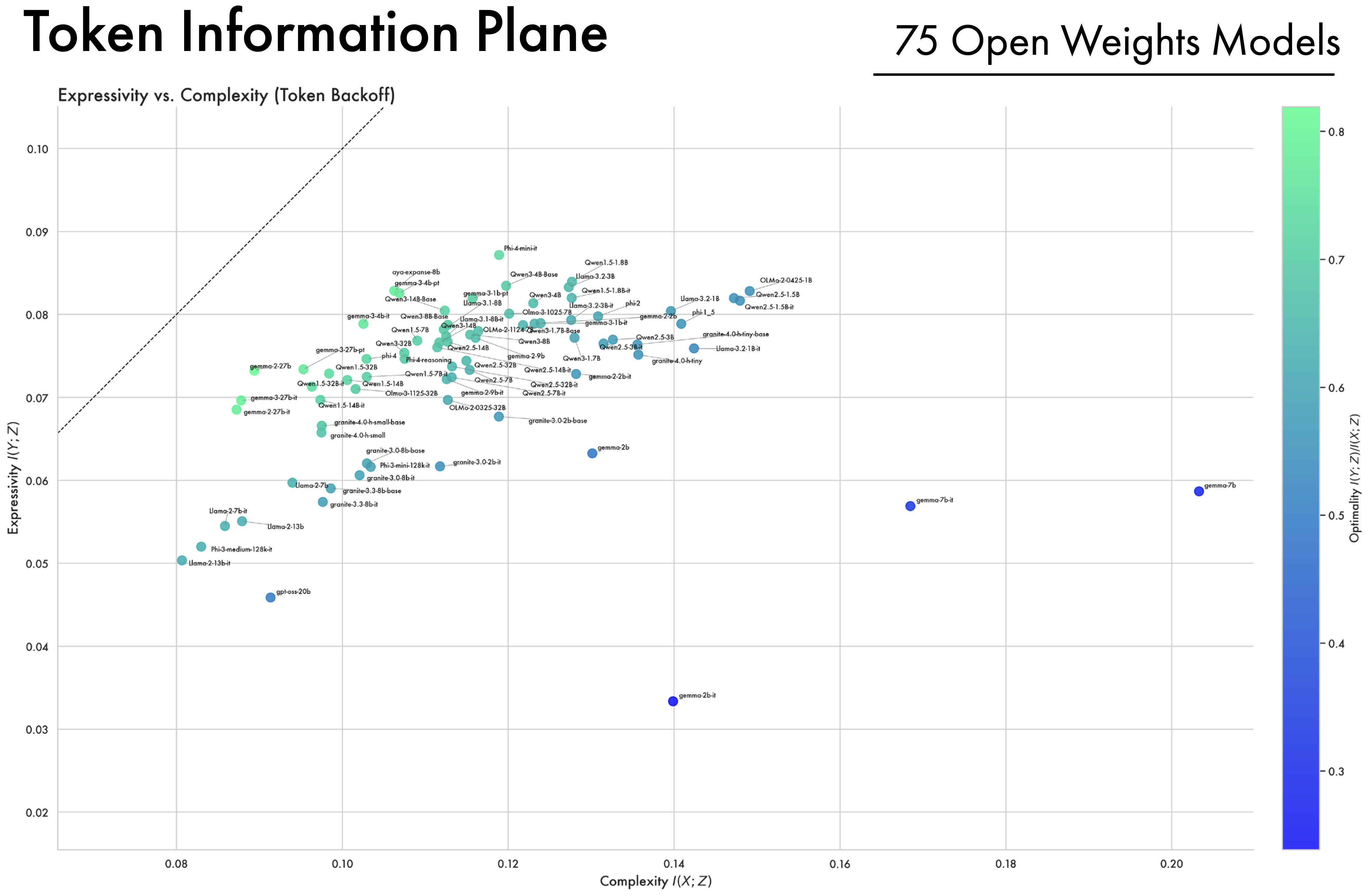
In order to study training time-courses our pre-training analyses look at the OLMo2 family of models (OLMo et al. 2025), which makes available intermediate checkpoints.4 We focus analysis on the 7B model unless otherwise noted, while including results for the 32B and 1B variants to show where conclusions hold or differ across model scales. In addition, to show our conclusions hold outside of this particular family of models we compare a wide array of open-weights LLMs (which do not make intermediate training checkpoints available), showing where they lie on the information plane at the end of training.
4 Appendix D includes additional pre-training analyses of the Smol LM2 (Allal et al. 2025) and Pythia (Biderman et al. 2023) models, which also make intermediate checkpoints available. These follow a similar pattern to the results presented here.
4.1 Pre-training Approaches Optimal Compression
The majority of pre-training appears to be a slow compression of a model’s training data. The Information Bottleneck theory of deep learning predicts two phases: a fitting phase during which output information \(I(Y;Z)\) increases, followed by a compression phase during which input information \(I(X;Z)\) decreases and representations approach the bound. This transition to compression is believed to occur when error on the training set saturates.
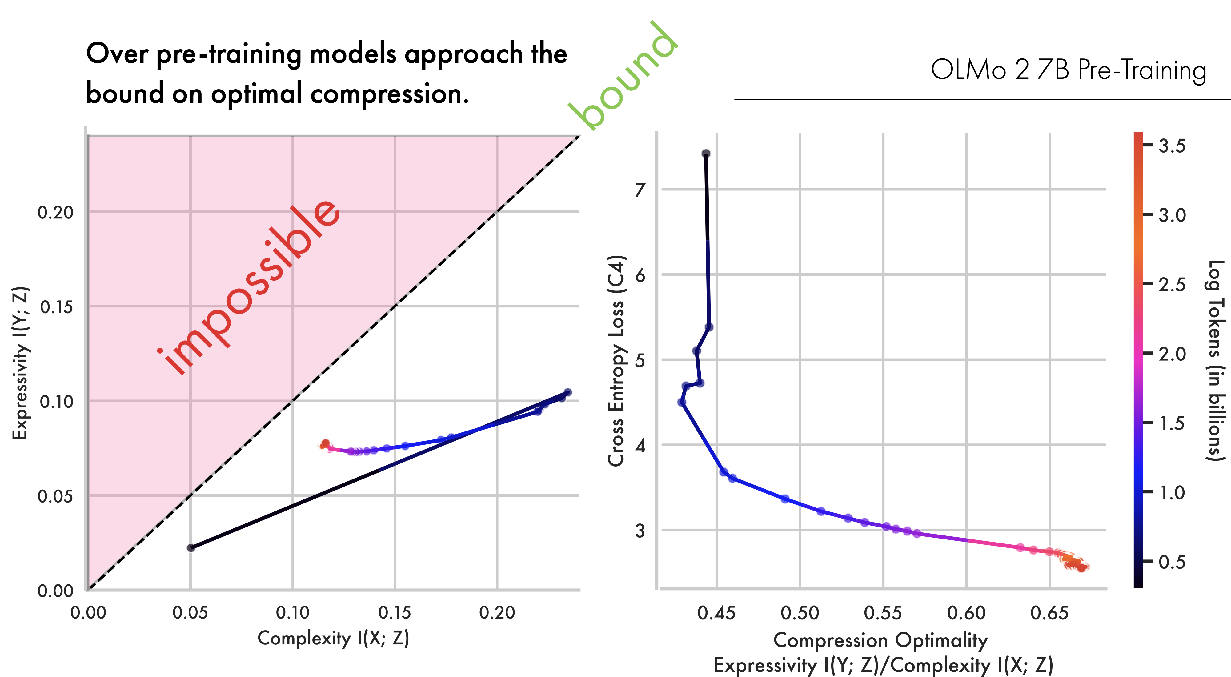
Shown in Figure 1 (and reproduced below) is the training trajectory for the OLMo2 7B model with respect to data from English C4. Strikingly, the 7B model closely follows the two-phase prediction from the Information Bottleneck, first increasing mutual information with outputs, before compressing input information and progressing towards the bound on optimal compression. Additionally this transition appears to happen as the model’s loss on next-token prediction begins to saturate. This shows how, even at scale, deep-learning models appear to thread a needle between representational complexity and expressivity. It also demonstrates how LLMs can be effectively studied from the perspective of Rate Distortion Theory, as they try to converge to an optimal lossy compression of their training data.
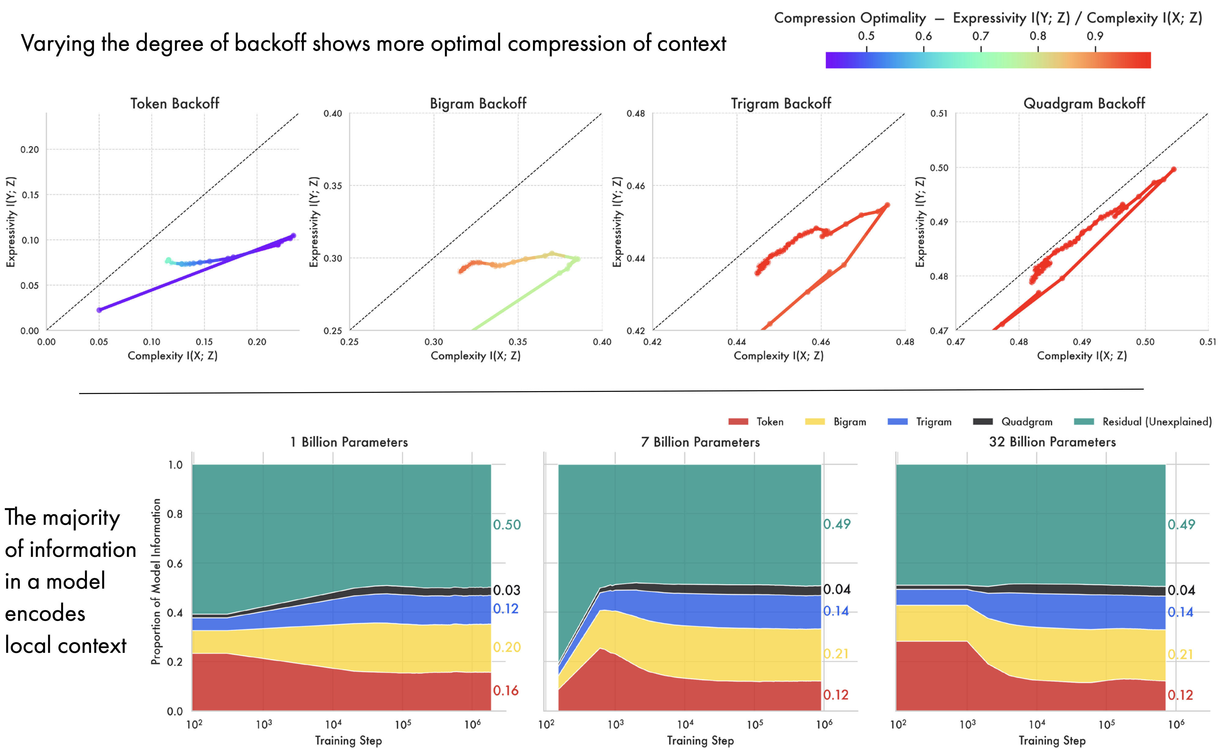
Models More Optimally Compress Contextual Information. By varying the degree of back-off in the source and target distributions used to compute mutual information, we can examine how contextual information evolves over pre-training at the token, bigram, trigram, and quad-gram levels. All cases result in a similar two-phase pattern of expansion and compression, with larger conditioning context converging closer to the bound. For token-level back-off late training aligns with previous work on MNIST (Shwartz-Ziv and Tishby 2017), with models compressing the source distribution — reducing complexity — while maintaining expressivity. At higher levels of contextualisation both complexity and expressivity are reduced. We hypothesise this is because in language modelling the source and target are sampled from the same distribution; what counts as an ‘input’ vs. an ‘output’ is a product of what point in the sequence the model is during generation. The higher degree of optimality in contextual encodings likely reflects an inherent pressure in the pre-training objective for models to develop representations of a token in context.
Embeddings Largely Encode Local Context. We compute the proportion of information in a model explained by each level of back-off in the source distribution independently. As shown in the figure above (bottom), the majority of information in a model encodes local context (token to quadgram), likely reflecting the information locality of the natural language on which they’re trained (Gibson 1998; Gibson et al. 2000; Hahn et al. 2022). The 1 billion parameter model also has more token information and less contextual information than its larger counterparts. The residual information likely encodes the finer-grained contextual distinctions found in the remainder of the 512 token context window — given the sparsity of n-grams greater than a quadgram those mutual informations are intractable for us to compute. This gives an interpretation of an LLM from the perspective of earlier work in NLP as akin to a context-window-width n-gram model that is smoothed enough to be tractable to train from finite data.
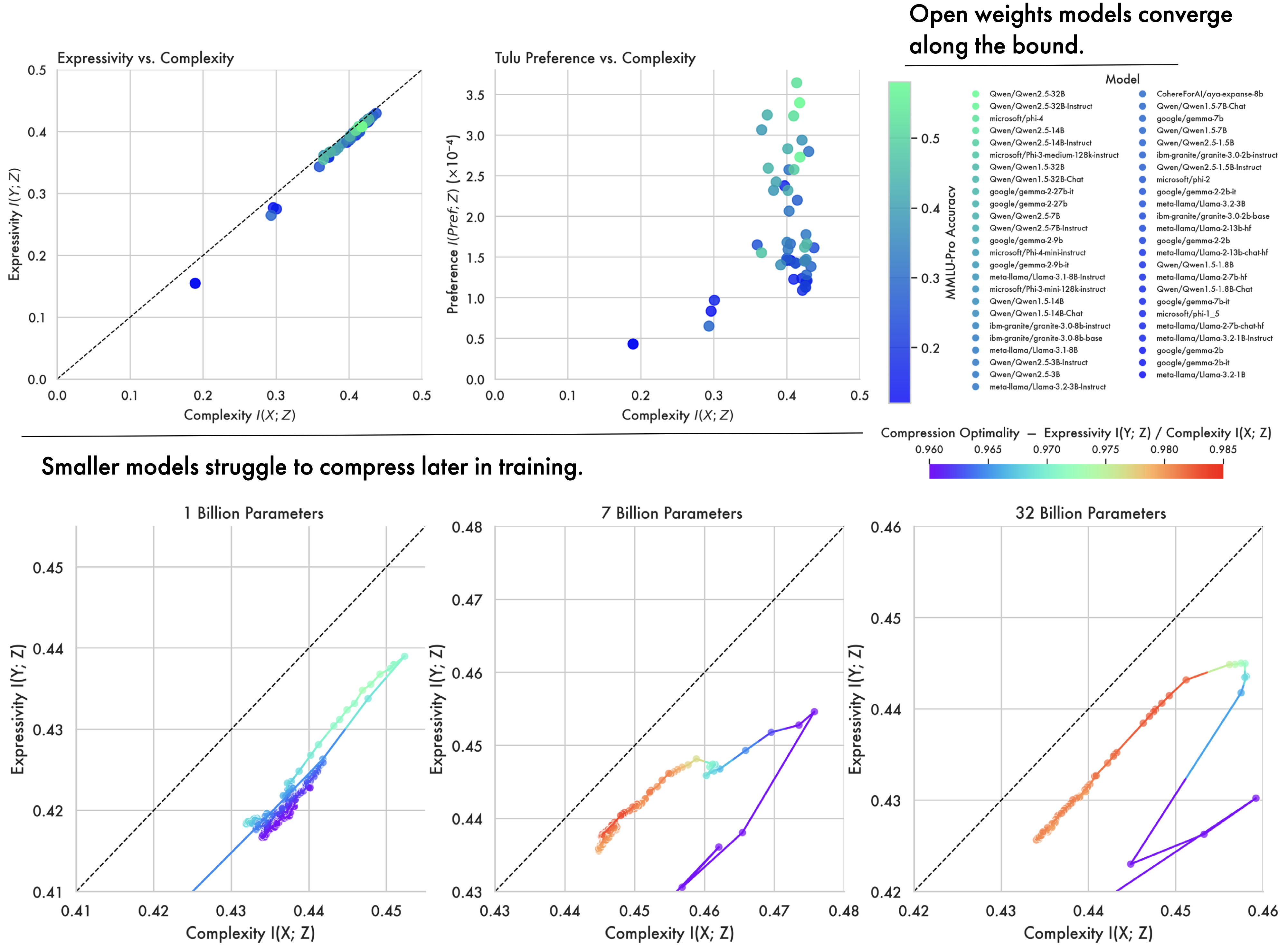
The Effect of Scale: Smaller Models Struggle to Compress. Parameter count shows a marked effect on the degree of compression achievable by a model. The larger models both closely follow the hypothesized Information Bottleneck trajectory, exhibiting phases of expansion and compression, ultimately approaching optimal compression. The 1B parameter model exhibits markedly different behaviour. While it successfully completes the initial expansion phase — increasing output information \(I(Y;Z)\) — it fails to approach optimal compression. Instead, in the second phase the smaller model oscillates while moving slowly away from the bound. This suggests that for a given level of data complexity, a certain parameter threshold may be necessary for models to achieve an optimal compression — an observation in line with work on scaling laws (Kaplan et al. 2020).
A Wide Array of Open-Weight Models Converge Along the Bound. In addition to looking at the OLMo2 family of models, we compute complexity and expressivity estimates across a diverse array of open-weight models. A striking convergence pattern emerges: across different model families, hyper-parameters, and training methodologies, representations ultimately converge and cluster near the bound on compression. Furthermore, models all approach the same point on the bound, suggesting they all converge to a similar information structure. This suggests that training as a process of compression is not an artifact of a single LLM’s training trajectory, but more fundamentally applies to deep-learning models as a class, and to the data and the objectives used to train them.
4.2 Relating Representation Structure to Performance
So far we have studied how information in an LLM is structured; we now consider how that structure relates to downstream performance. We look at how representational information for 47 open weights models from 6 different families relates to performance across six benchmarks (Fourrier et al. 2024): MMLU Pro, BBH, Math LVL5, IFEval, GPQA, and MuSR.
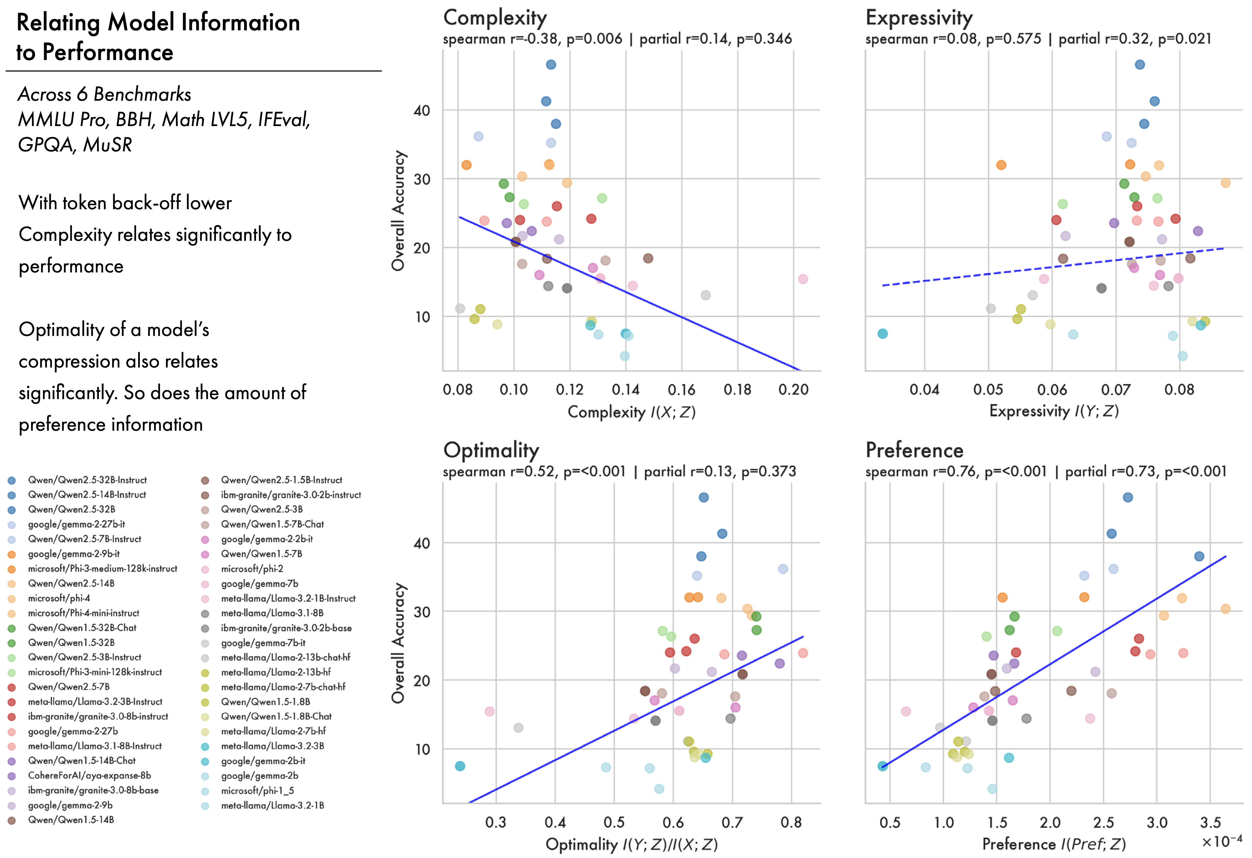
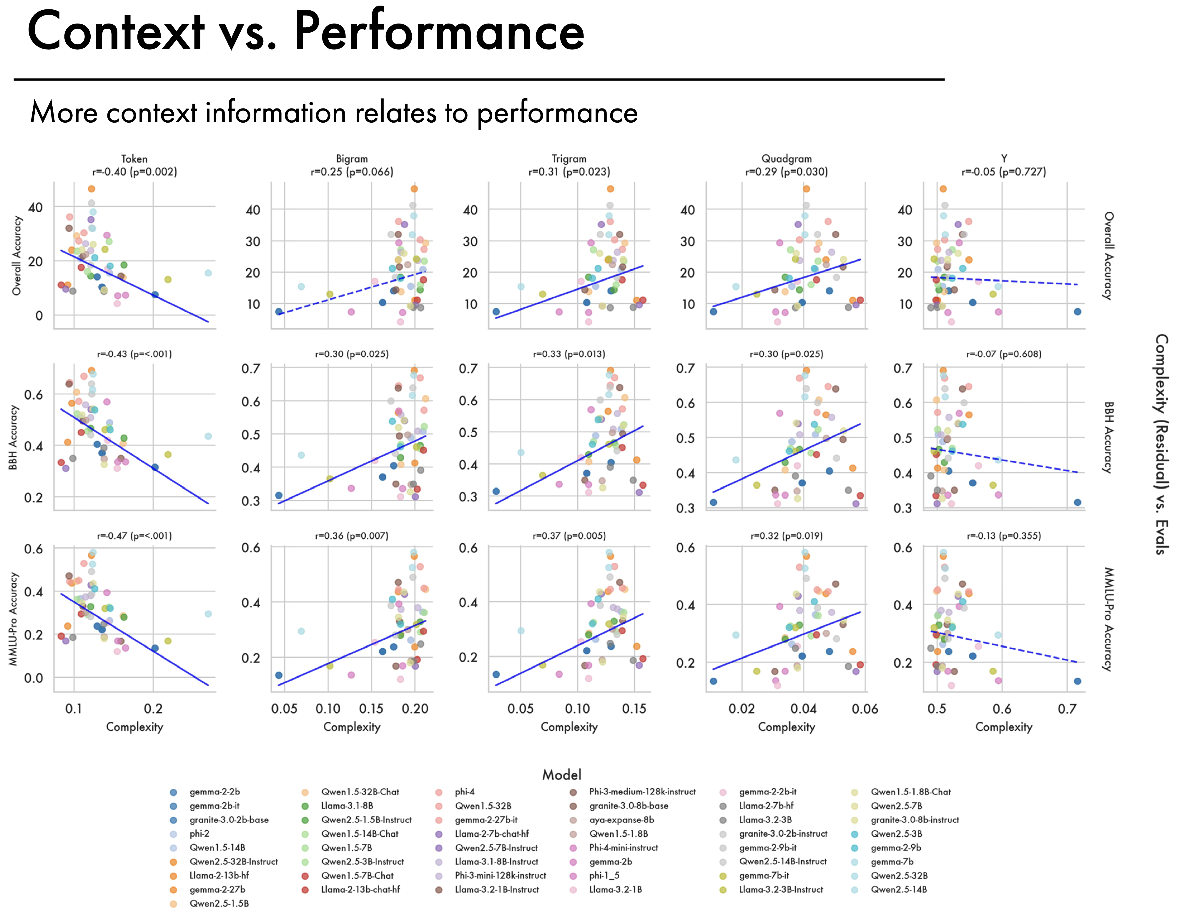
At the token level, lower complexity relates significantly to performance (\(r=-0.38\), \(p=0.006\)), while expressivity alone does not (\(r=0.08\), \(p=0.575\)). However, the ratio between expressivity and complexity — a measure of how close a model is to optimal compression — is a significant predictor of downstream performance (\(r=0.52\), \(p<0.001\)). This tells us that better performing models have less token complexity, and are more optimally compressed.
More Contextual Information Improves Performance. Looking beyond token-level backoff we see a pattern emerge. Proportionally less token information correlates with downstream performance but having more bigram, trigram, and quadgram information correlates positively with performance. Intuitively this shows how models that have a better representation of context, allocating less of their representations to token-level distinctions, perform better downstream. This aligns with our finding that larger models allocate more of their representation space to contextual information.
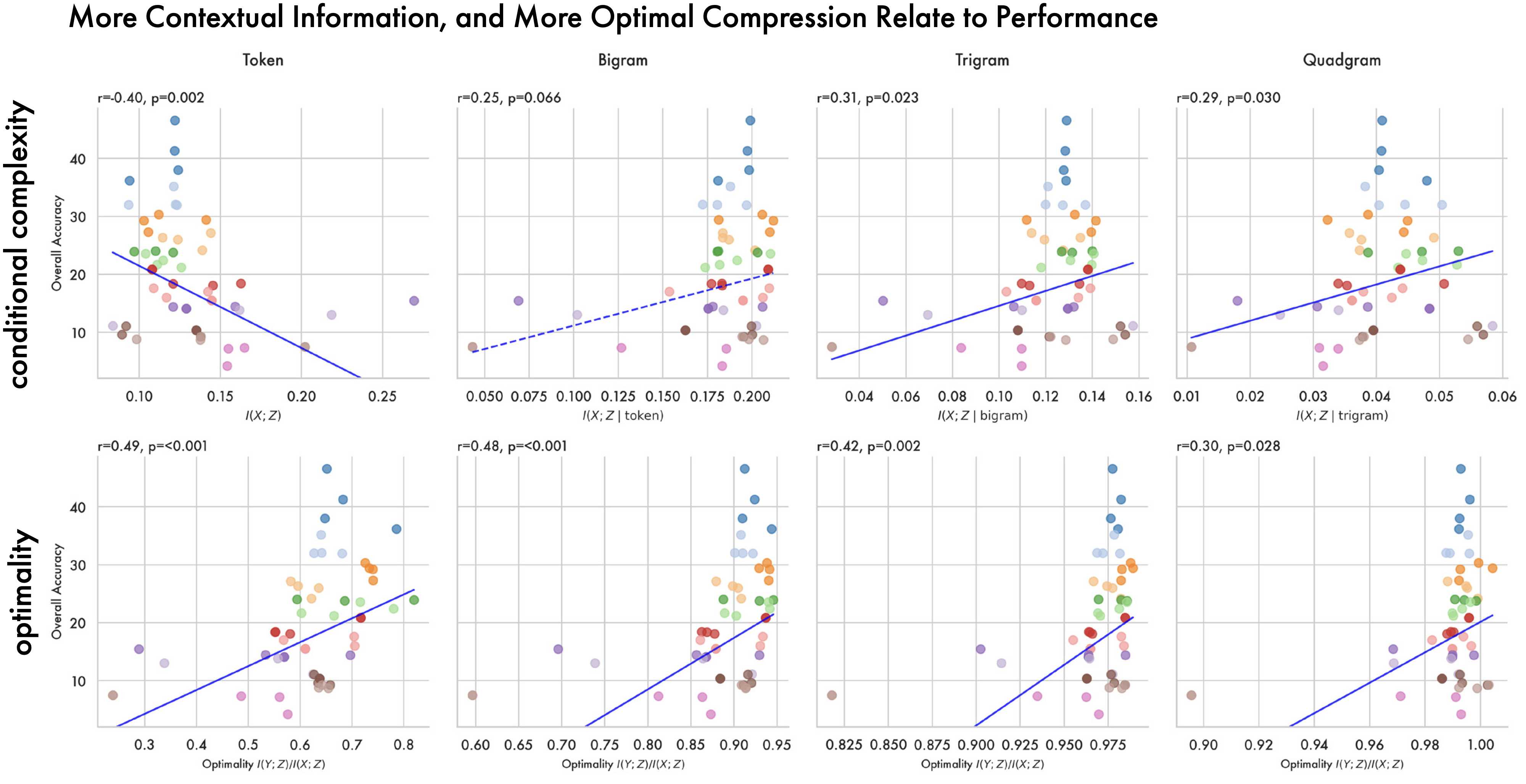
Optimal Compression. At all levels of back-off we see a consistent relationship between how close a model is to the information bottleneck bound on compression, and its performance downstream. Closer to the bound, representations preserve only the information from the input that is relevant to predicting the output. While higher performing models have more context information and less token information, how close to the bound representations are at each level of context is consistently positively related to performance. This allows us to link the simplest representation, at a given level of expressivity, to the most generalisable representation across the benchmarks considered here. Critically these compression estimates are computed with general data from the internet (C4) rather than data from the evaluations themselves, showing our methods can identify sufficiently general properties of a compression that we can predict downstream performance without knowledge of the test distribution.
Preference. While LLMs approach optimal compression for next sequence prediction over pre-training, a large body of work also tries to improve their ability to follow instructions, and generate responses humans prefer (Ouyang et al. 2022). We use preference data (Lambert et al. 2024) to compute mutual information with preference. The amount of preference information in a model proves a significant predictor of downstream performance (\(r=0.76\), \(p=0.001\)). This suggests that not only does the optimality of a model’s compression matter, but exactly what information survives that compression does too. In Appendix B we include results showing that post-training can increase the amount of preference information across different models in two different families while minimally changing their complexity. This suggests that pre-training is responsible for the broad compression learned by a model, while post-training edits the information it contains.
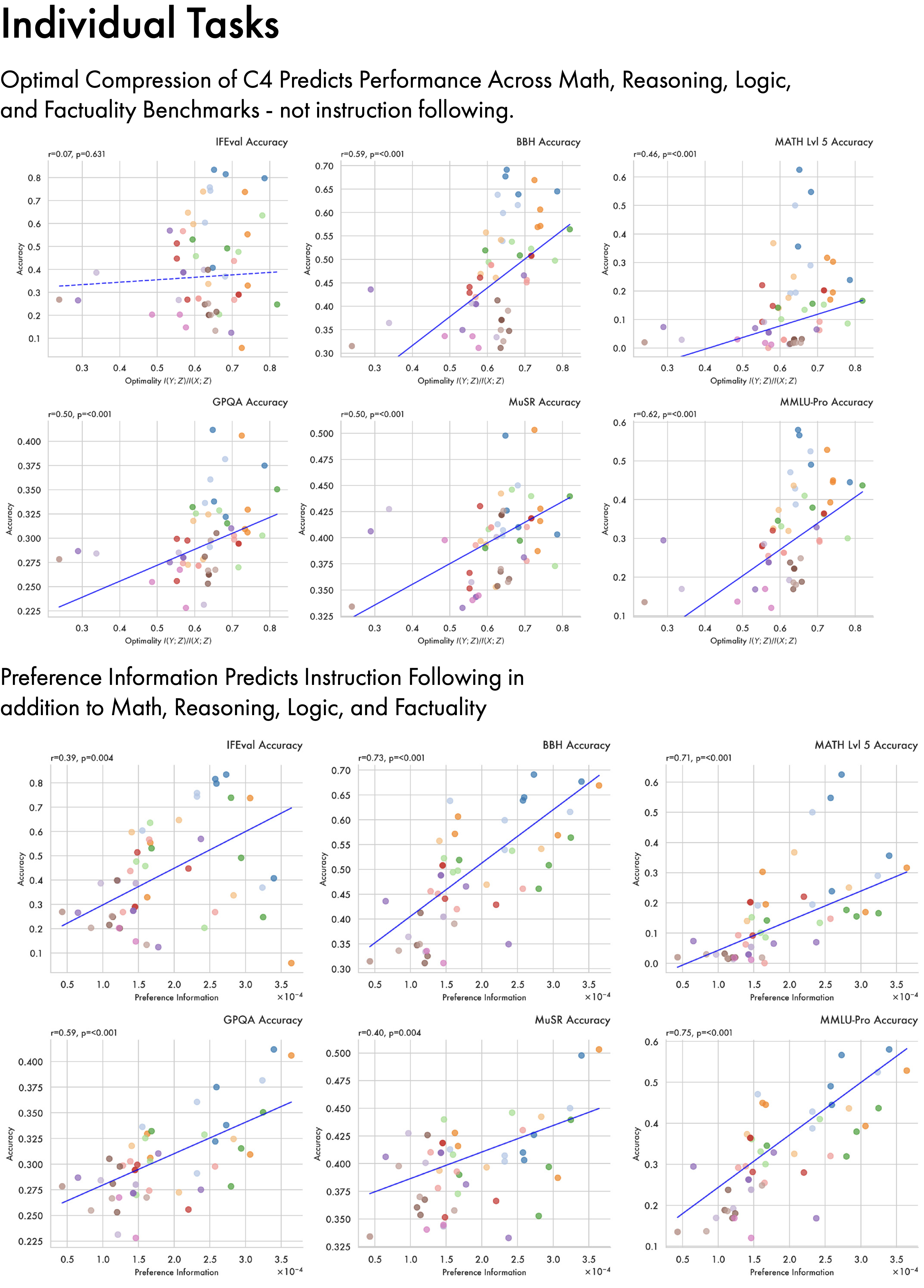
Results here focus on aggregate performance across 6 benchmarks; in Appendix C we discuss each of the benchmarks individually. At the individual task level optimal compression of C4 significantly predicts performance across math, reasoning, and factual knowledge benchmarks — but not instruction following. Instruction following is, however, predicted by the amount of preference information in a model. This helps us better understand what behaviours optimal compression of C4 is likely to give rise to — like broad factual knowledge — and what it is unlikely to give rise to, e.g. the ability to respond to questions with precise formatting and word counts.
More broadly these results indicate how the information theoretic approach taken here could potentially be leveraged during training. Optimality could be used as a stopping-criterion — ceasing pre-training when distance to the bound no longer decreases — or as a model-selection criterion — picking the checkpoint that is the most optimally compressed, or with the highest proportion of preference information. Given the estimates here are computed with a single-forward pass using teacher forcing, computing an entropy estimate for candidate selection would be substantively less costly than evaluating a model across a suite of benchmarks.
5 Conclusion
The work presented here bridges the gap between theoretical accounts of learning and the practical complexities of LLMs. We show that LLMs learn an optimal compression of the data on which they are trained, with a wide array of open-weights models converging along the IB bound — with the optimality of a model’s compression predicting downstream performance. Each compression is different; we can account for the information that survives the compressive process, showing how representations encode information about different levels of local context and human preferences.
The approach to interpretability we introduce here interprets a model as a whole — rather than focussing on a particular circuit, or attention head, or representational measures for just the final embedding from the final layer — because complex distributed systems are not best understood in terms of their parts alone. Giving a holistic account of what it means to train an entire model on the entire internet is a challenge, but we argue that LLMs are best understood as lossy compression. In doing so, we place them in the context of a long history of work on representation learning across the sciences.
A — Open-Weights Models, Detailed Visuals
B — Post-Training and Preference Information
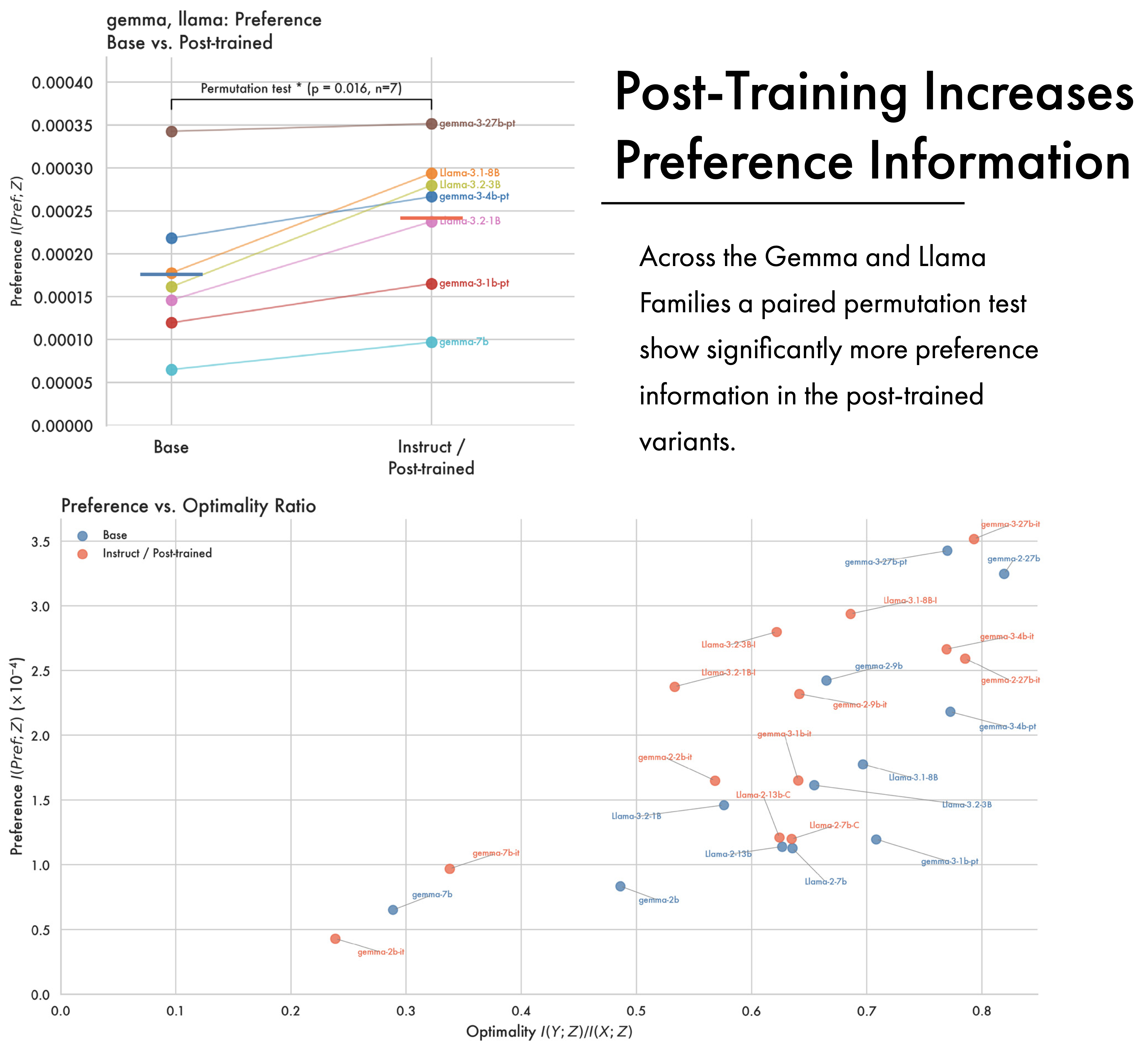
While LLMs become optimally compressed for next sequence prediction over pre-training, the final phase of the training pipeline often introduces other kinds of information. In the general case, post-training is designed to improve a model’s ability to follow instructions and better align it with human preferences; we look at how this changes the information content of a model, and how it affects the representations from pre-training. The figure above shows preference information across two different families of open weights models, Llama and Gemma, which release a checkpoint at the end of pre-training and one at the end of post-training. In the Llama case post trained models consistently have higher preference information than their pre- and mid-trained counterparts. This supports a framing of pre-training as imbuing the model with core semantic information, which is later augmented with task-specific and preference information. With the Gemma models the picture is more complicated, with a consistent effect for the most recent Gemma 3 release — post trained models have greater preference information — but no significant pattern across earlier models.
C — Predicting Performance on Individual Tasks
In the main paper we focus analysis relating representational structure to performance on aggregate performance across 6 benchmarks.
IFEval (Zhou et al. 2023): A benchmark of approximately 500 prompts containing objectively verifiable constraints such as word counts, keyword inclusion, and formatting requirements. Strong performance indicates that a model can reliably adhere to precise, compositional instructions rather than merely producing plausible text.
MMLU-Pro (Wang et al. 2024): An enhanced multi-task language understanding benchmark containing over 12,000 questions across 14 domains with ten answer choices per question. It emphasizes reasoning-focused questions over pure knowledge recall. Strong performance indicates broad expert-level knowledge and robust reasoning across STEM, humanities, and social sciences.
BBH (Suzgun et al. 2022): A suite of 23 challenging tasks drawn from BIG-Bench on which prior language models failed to outperform average human raters. Tasks span algorithmic, logical, commonsense, temporal, and multi-step reasoning. Strong performance indicates the ability to carry out diverse, non-trivial reasoning that benefits from chain-of-thought prompting.
MATH Level 5 (Hendrycks et al. 2021): The hardest difficulty tier of the MATH dataset, which contains competition-level mathematics problems sourced from contests such as the AMC and AIME. Strong performance indicates the ability to solve multi-step problems requiring creative mathematical reasoning, not just computation.
GPQA (Rein et al. 2024): A set of 448 graduate-level multiple-choice questions in biology, physics, and chemistry, written by PhD-level domain experts. The questions are designed to be “Google-proof” — skilled non-experts with full web access achieve only ~34% accuracy. Strong performance indicates deep scientific reasoning beyond surface-level retrieval.
MuSR (Sprague et al. 2024): A benchmark of multistep soft reasoning tasks embedded in natural-language narratives (e.g., ~1000-word murder mysteries). It requires extracting facts, applying commonsense, and chaining multiple inference steps. Strong performance indicates robust narrative comprehension and multi-hop reasoning in realistic settings.
Here analysing the individual task correlations reveals a pattern. Optimal compression of C4 — a broad crawl of the internet — predicts performance across math, reasoning, and factuality benchmarks, but not IFEval (\(r=0.07, p=0.631\)). IFEval assesses a model’s ability to follow specific compositional instructions in the prompt, and performance here is predicted by the amount of preference information present in a model (\(r=0.39, p=0.004\)). This sheds light on what drives model performance: general purpose knowledge and reasoning is related to optimal compression of the training data, while instruction following is related to preference information which arises during post-training. Preference information proves predictive of math, reasoning, and factuality benchmarks as well as instruction following — but this may largely reflect the makeup of the preference data used.
D — Additional Model Timecourses
A major challenge in studying pre-training is the limited availability of checkpoints. We focus analysis in the main paper on the OLMo2 models as they offer comprehensive checkpointing and comparatively strong performance. Here we look at two other families of models which make available some pre-training checkpoints.
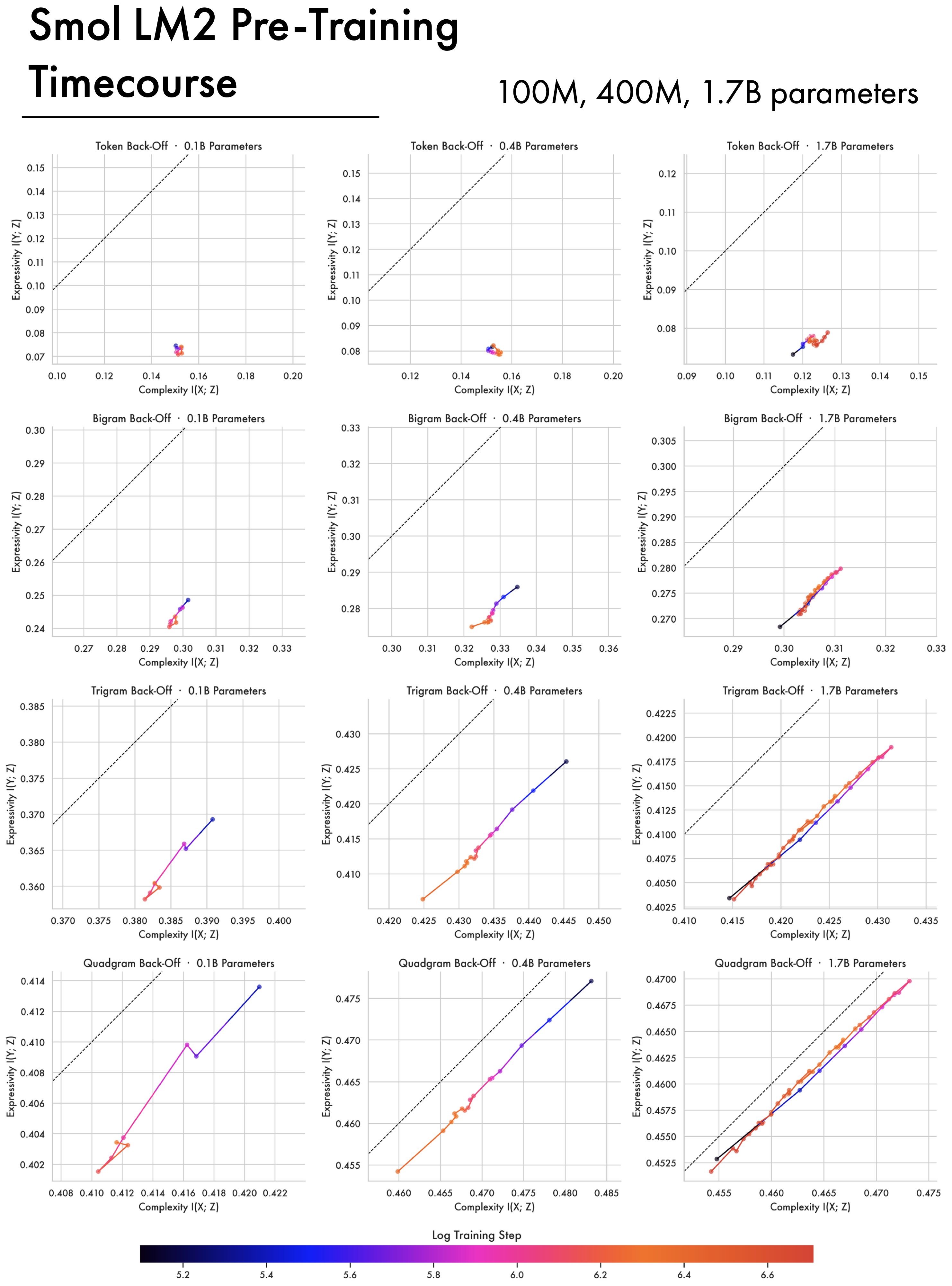
The Smol LM2 models (Allal et al. 2025) are models with 1.7B parameters or smaller that achieve competitive performance. The 1.7B Smol model was trained on 11 Trillion tokens and performs comparably to the 1B OLMo2 model which was trained on 4 Trillion Tokens. Broadly the 1.7B Smol model follows a similar training trajectory to the OLMo2 1B model, having phases of expansion and compression but failing to approach the bound like the OLMo2 7B and 32B models. This figure also includes trajectories for the smaller 100M and 400M variants — these models struggle to show much meaningful compression, though part of the issue may be that checkpointing starts comparatively late in the pre-training process.
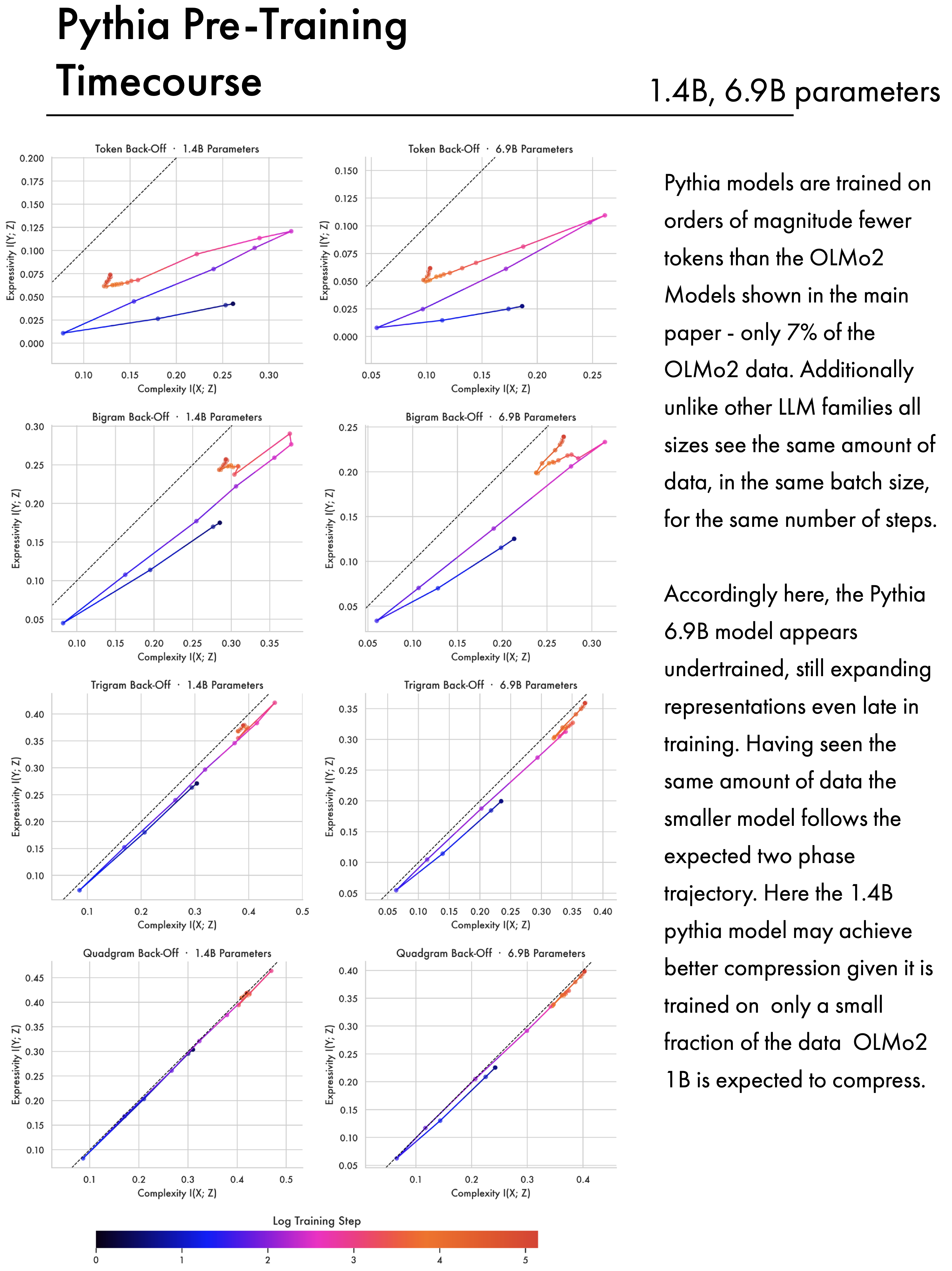
The other family of models we analyse are the Pythia models (Biderman et al. 2023). Included are analyses of the 1.4B and 6.9B models. In terms of parametrisation these are roughly comparable to the 1B and 7B OLMo2 models analysed in the main paper. However the methodology for training these models is substantially different, and their performance is substantially lower than the OLMo2 models. Pythia models are intended for scientific analysis — as a result they use the same amount of data, batch size, and number of training steps across model sizes, and are trained on the Pile dataset (L. Gao et al. 2020). This contains roughly 300 billion tokens; by contrast the 1B OLMo2 model is trained on 4 trillion tokens — meaning the Pythia models see 7.5% of that data. Accordingly the 1.4B Pythia model appears to achieve better compression later in training than its OLMo counterpart. The 6.9B Pythia model is still expanding representations late into pre-training, suggesting it is under-trained.
E — Entropy Estimation
E.1 — Estimator Hyperparameters
The estimator has two parameters that need to be set: the number of bins \(m\) and the temperature used in the softmax \(\varepsilon\). As shown in Appendix E.8 and Conklin (2025), the estimator is generally robust with respect to the number of bins — in all experiments presented here we use \(m=100\).
Temperature Calibration
Naively we could use the same temperature across all models, however models differ in the dimensionality of their hidden representations. Within self-attention, as the dimensionality \(d_k\) of query and key vectors grows, the variance of their dot products scales linearly with \(d_k\), pushing the softmax function into saturated regions where gradients vanish (Vaswani et al. 2017). This is a specific instance of the broader concentration of measure phenomenon in high-dimensional spaces, where distance and similarity metrics become increasingly uniform and less discriminative (Aggarwal, Hinneburg, and Keim 2001). As a result Vaswani et al. (2017) scales the dot product by \(\sqrt{d}\) to avoid saturation.
The soft entropy estimator uses dot-products on the surface of the unit hypersphere passed through a softmax in order to estimate a density. As a result, for a fixed temperature, higher-dimensional space will begin to appear more uniformly distributed. We compute a temperature which is calibrated to prevent saturation, making estimates for different dimensionalities directly comparable.
Let \(V_\varepsilon\) denote the von Mises–Fisher (vMF) distribution on unit hypersphere \(\mathbb{S}^{d-1}\) with concentration parameter \(1/\varepsilon\); by rotational symmetry, \(D_{\mathrm{KL}}(V_\varepsilon \| U)\) depends only on \(\varepsilon\) and \(d\), and measures how far a single vMF kernel is from uniform. For an arbitrary data distribution \(P\) on the sphere, let \(P_\varepsilon\) denote the convolution of \(P\) with the vMF kernel at temperature \(\varepsilon\); the smoothed KL divergence \(D_{\mathrm{KL}}(P_\varepsilon \| U)\) is the estimation target, and satisfies \(0 \leq D_{\mathrm{KL}}(P_\varepsilon \| U) \leq D_{\mathrm{KL}}(V_\varepsilon \| U)\) by Jensen’s inequality.
For the soft entropy estimator \(\widehat{D}^{(\mathrm{SQ})} = D_{\mathrm{KL}}(\hat{p} \| u_m)\) takes values in \([0, \log m]\), where \(m\) is the number of bins. To ensure this range is well-matched to the estimation target, we calibrate the temperature \(\varepsilon\) so that the maximum possible value of the target equals \(\log m\). The target is bounded above by \(D_{\mathrm{KL}}(V_\varepsilon \| U)\). Direct computation requires evaluating modified Bessel functions, which is numerically unstable at large \(d\); however, using Amos-type bounds on Bessel function ratios (Amos 1974), one can construct upper and lower envelope functions \(\Psi^\pm_{\varepsilon,d}\) satisfying \(\Psi^-_{\varepsilon,d} \leq D_{\mathrm{KL}}(V_\varepsilon \| U) \leq \Psi^+_{\varepsilon,d}\), with a gap of order \(O(d^{-1})\). It can be shown that \(D_{\mathrm{KL}}(V_\varepsilon \| U)\) is monotone decreasing, so the equation \(D_{\mathrm{KL}}(V_\varepsilon \| U) = \log m\) has a unique solution \(\varepsilon^\star(m,d)\). To leading order in \(d\):
\[ \varepsilon^\star(m, d) \approx \frac{1}{\sqrt{2d \log m}} \]
Throughout our experiments, we use the more exact bounds, \(\Psi_{\varepsilon, d}^{\pm}\), to calibrate temperature. These bounds are numerically stable in high dimensions, and we approximate \(\varepsilon^\star(m,d)\) by choosing the smallest temperature \(\varepsilon\) such that \(\Psi_{\varepsilon, d}^+ \leq \log m\). In practice this is computed once per model based on \(m=100\) and the model’s dimensionality. The correction here bears strong resemblance to the default scaling within self attention \(\sqrt{d}\).
E.2 — Approximating the Input Distribution
We estimate the mutual information between model inputs and outputs. In an auto-regressive decoder-only LLM the input to a model is the preceding context up to the current token. We view the input as n-grams of tokens where the input at timestep \(x_t\) is an ngram of width \(t\) containing all tokens \(x_0 \ldots x_t\). Maintaining probability distributions for every possible context proves intractable due to the combinatorial complexity of natural language. Additionally, ngrams greater than 3 tokens become sparsely distributed in the data making reliable estimation of their probabilities a challenge. As a result we condition estimates on ngrams of fixed-widths 1, 2, 3, 4 — referred to in the paper as token, bigram, trigram, quadgram. This is related to Backoff (Katz 1987) which reduces n-gram size until the n-gram has non-zero probability in a corpus. Here though we do not interpolate different n-gram widths, instead maintaining separate aggregate estimates for each width — in part to be able to study how different levels of contextual information are represented in the model. Where a given n-gram, like a quadgram, does not have non-zero probability in the data it is omitted from the overall quadgram mutual information estimate.
In practice this means estimates for smaller n-gram widths are more reliable — a classical issue in language modelling (Jurafsky and Martin 2000, 32). Token, bigram, and trigram estimates can be estimated reliably from a relatively small sample of data. We judge this by looking at how estimates change as a function of the number of samples during the estimation procedure; by 5,000 samples these estimates reliably begin to converge. Quadgrams, due to their sparsity, tend to have less robust estimates. As a result our broad comparison of open-weights models uses token and bigram estimates. The pre-training model size analysis focuses on trigram estimates as the widest context that still reflects a reliable estimate. The analysis of how context is represented over pretraining includes quadgram estimates for reference.
E.3 — Approximating the Output Distribution
During inference models predict the next token given preceding context, but this is distinct from how they are trained. During training of an auto-regressive decoder-only LLM, causal masking means a token can only attend to preceding context. However transformer decoders are trained using teacher forcing, where predictions are generated for the entire sequence in parallel by assuming predictions are made correctly — this is distinct from having training operate one token at a time. The result is that for an embedding \(e_t\) at timestep \(t\), following embeddings \(e_{t+1}\) can attend to \(e_t\). This means embeddings get gradient information from the trailing context.
Given that our analysis computes embedding mutual informations over training with respect to a model’s input and outputs, this has implications. It means that the output for \(e_t\) is not just \(y_{t+1}\) but all following output tokens \(y_{t+1} \ldots y_{n}\) where \(n\) is the sequence length. As a result we consider \(X\) to be the entire preceding context in the input, and \(Y\) to be the entire trailing context after the current point in the sequence. This means when we compute mutual informations for different n-gram widths we match the width for \(X\) and \(Y\) — conditioning the estimates on the same width of preceding and trailing context respectively.
E.4 — Estimating Mutual Informations
To compute mutual informations between the input \(X\) and representations \(Z\), we need two quantities: the entropy of representations \(\mathcal{H}(Z)\) and the conditional entropy given the input \(\mathcal{H}(Z|X)\). To compute \(\mathcal{H}(Z)\) we use the quantisation procedure described in Section 3.1 applied to all token embeddings, giving \(\hat{Z}\) — by summing over each embedding and renormalising we get a categorical distribution \(P(Z)\) that describes the embedding space. To get a conditional estimate \(P(Z|X)\) we simply take \(\hat{Z}\) and compute a subset containing the embeddings corresponding to the input \(X\), \(\hat{Z}|X\). Summing and renormalising gives us \(P(\hat{Z}|X)\).
This brings us to an important distinction: our analysis discusses mutual informations with respect to tokens, bigrams, trigrams, and quadgrams. These are not computed over different widths of embeddings, but rather over single token embeddings conditioned on the preceding context. It means that \(Z|\text{token}\) is a subset of \(Z\), \(Z|\text{bigram}\) is a subset of \(Z|\text{token}\), \(Z|\text{trigram}\) is a subset of \(Z|\text{bigram}\), etc. The terms token, or bigram mutual informations refer to the width of the conditioning context, not the width of the embeddings over which entropy is computed.
E.5 — Conditional Mutual Informations and the Residual
In order to compute what proportion of a model encodes each level of context we use the chain rule for mutual information. As we increase the context width used in back-off the estimates contain each other — the bigram mutual information includes the token mutual information. The chain rule means:
\[ I(X; x_t, x_{t-1}) = I(Z; x_t) + I(Z; x_{t-1}|x_t) \]
which allows us to separate out the information explained by the current token \(I(Z;x_t)\) and the preceding one given the current token \(I(Z; x_{t-1}|x_t)\). For the source distribution \(X\) and a given n-gram width \(n\) we can get a proportion \(\phi\) of model information by normalising by the entropy of the model:
\[ \phi(x, n) = \frac{I(Z; x_{n}|x_1 \ldots x_{n-1})}{\mathcal{H}(Z)} \]
We compute this for each level of backoff, where at the token level \(\phi(x, 1) = I(Z;x_t)/\mathcal{H}(Z)\). The most granular label we have is quadgram. The residual, or unexplained information, is the information in the model left after subtracting the mutual information of the most granular category:
\[ \phi_{\text{residual}}(x, n_{\max}) = \mathcal{H}(Z) - I(Z; x_n \ldots x_{n_{\max}}) \]
E.5.1 — Conditional Mutual Informations and Performance
Shown above — less token information, but a higher proportion of local contextual information, relates significantly to downstream performance. In the main paper we report token level back-off in the correlation results, where lower complexity is related to performance.
E.6 — On The Use of Shannon Entropy
In this paper we compute the entropy of continuous latent variables. As a result it is natural to ask why we — in line with previous work (Shwartz-Ziv and Tishby 2017; Voita, Sennrich, and Titov 2019; Sajjadi et al. 2018) — opt instead to discretise representations and compute their Shannon entropy (Shannon 1948). There are two major reasons for this. First, differential entropy is not the true continuous analogue of Shannon Entropy (Jaynes 1957). This is shown by the fact that differential entropy \(D(X)\) is unbounded \(-\infty \le D(X) \le \infty\), and variant under linear transformations. This is the main motivator for an information theoretic analysis to discretise and use Shannon entropy directly. A secondary consideration is that we don’t know how embeddings are distributed, so in order to get a differential entropy estimate we would first need to fit a distribution to the data. At scale this fitting step can be expensive, and introduce topographic assumptions.
E.7 — Scalability of Prior Work
Shwartz-Ziv and Tishby (2017) perform an empirical information theoretic analysis of neural-networks trained on MNIST. To do so they perform dimension-wise discretisation of model embeddings. This turns a 16-dimensional vector into a 16 character string. They then convert this to a categorical distribution over all possible strings. This approach works well on small problems, but the dimension-wise discretisation requires taking a hidden representation with dimensions \(\textit{batch}\times\textit{hidden}\) and transforming it to \(\textit{batch}\times\textit{hidden}\times\textit{n bins}\). If using 50 bins, in practice this means using 50 times the memory of not discretising. For the OLMo2 32B model used in this paper which has a hidden dimension of 5120 and 64 layers, and where we have a context window of 512 tokens, this would require holding in memory a tensor of dimensions \(\textit{batch}\times 512\times5120\times64\times\textit{n bins}\). The memory use of this approach makes it intractable to apply to contemporary models.
Voita, Sennrich, and Titov (2019) studied the transformer base model which has only 6 layers with a hidden dimension of 512. Despite this they note the approach from Shwartz-Ziv and Tishby (2017) was not tractable to apply to the model. They opt instead for quantising representations via clustering, based on related work from Sajjadi et al. (2018). This method runs a clustering algorithm (mini-batch k-means), then treats each cluster as an event in a categorical distribution. While this method provides robust entropy estimates and dramatically less memory usage, it still has relatively high computational complexity. It requires running a clustering algorithm to convergence before performing quantisation, prohibiting its use in an online setting. Again thinking of the OLMo2 32B model used here, this would require running a clustering algorithm on 5120 dimensional spaces, at all 64 layers separately, for each of the 150 pre-training checkpoints. This would provide the ‘bins’ for the quantisation, then embeddings would need to be assigned to bins, requiring a second forward pass.
In practice an information-theoretic analysis of an LLM requires an entropy estimation method that is memory efficient, fast to compute, and can be applied in an online setting — requiring a single forward pass and no caching of the embeddings. The only estimator we’re aware of that meets these criteria is the soft-entropy estimator (Conklin 2025). Here the quantisation requires only a cosine-similarity and a softmax, making it fast and memory efficient. Additionally the normalisation step means ‘bins’ can be computed once at the start of the analysis, rather than needing a pass through the data to fit clusters. Conklin (2025) notes that the use of cosine similarities means this method considers only angular information in the representation space. However use of cosine-based methods is standard practice in NLP (Zhang et al. 2020; Reimers and Gurevych 2019; T. Gao, Yao, and Chen 2021), with some work suggesting vector norms in LLMs predominantly encode frequency information (Oyama, Yokoi, and Shimodaira 2023).
E.8 — The Information Bottleneck Bound
The Information Bottleneck bound is the curve traced by varying the trade-off parameter \(\beta\) in:
\[ \mathcal{F}_\beta[p(Z|X)] = I(X;Z) - \beta I(Y; Z) \]
The curve this traces is where representations are optimally compressed. Along this bound \(p(Z|X)\) is an optimal encoder, preserving only the information in \(X\) relevant to \(Y\). For a given dataset this optimal encoder can be found numerically via a version of the Blahut-Arimoto (Blahut 1972; Arimoto 1972) method for computing channel capacity. Introduced in Tishby, Pereira, and Bialek (2000), the information bottleneck method relies on three equations:
\[ p_{\beta}(z|x) = \frac{p_{\beta}(z)}{Z_{\beta}(x)}\exp\!\biggl(-\beta\, D[p(y|x)\|p_{\beta}(y|Z)]\biggr) \]
\[ p_{\beta}(z) = \sum_{x\in X}p(x)p_{\beta}(z|x) \]
\[ p_{\beta}(y|z) = \sum_{x\in X}p_{\beta}(x|z)p(y|x) \]
These equations are satisfied self-consistently at the bound. As these three equations rely on each other, one can learn an optimal encoder by starting with a randomly initialised one and iteratively computing each equation in turn.
In the general case the shape of this bound follows a linear relationship, until all mutual information between \(x\) and \(y\) is captured. At this point the curve saturates — additional complexity doesn’t result in additional accuracy, as there’s no more predictive information in \(x\). Numerical computation of the bound in our setting proves intractable. The optimal encoder \(p(z|x)\) needs to map all of natural language to representations that optimally predict the next token. In experiments we are able to compute a bound for tokenizers up to 50,000 tokens, however past this point convergence begins to fail. Given that we would like to have a bound for problems where numerical computation proves intractable, we leverage the observed linear pattern — the bound follows a linear relationship until the saturation point where \(I(Z;Y)=I(X;Y)\). Across all open weights models the highest token complexity converged to is 0.15, well below the saturation point. This is in line with results from Shwartz-Ziv and Tishby (2017), which shows FFNs on MNIST only converge near the saturation point when over-fitting.
F — Relating Compression to Training Loss
Prior work (Shwartz-Ziv and Tishby 2017) shows that models transition from the fitting phase to the compression phase when empirical error on the training distribution saturates. Their setting is substantively different to the one studied here — the most relevant differences are that they analyse a feed-forward model trained on MNIST for multiple epochs, meaning the model’s performance can fully saturate in-distribution. In an LLM setting models are trained on orders of magnitude more data, often for a single epoch, meaning saturation is more graded.
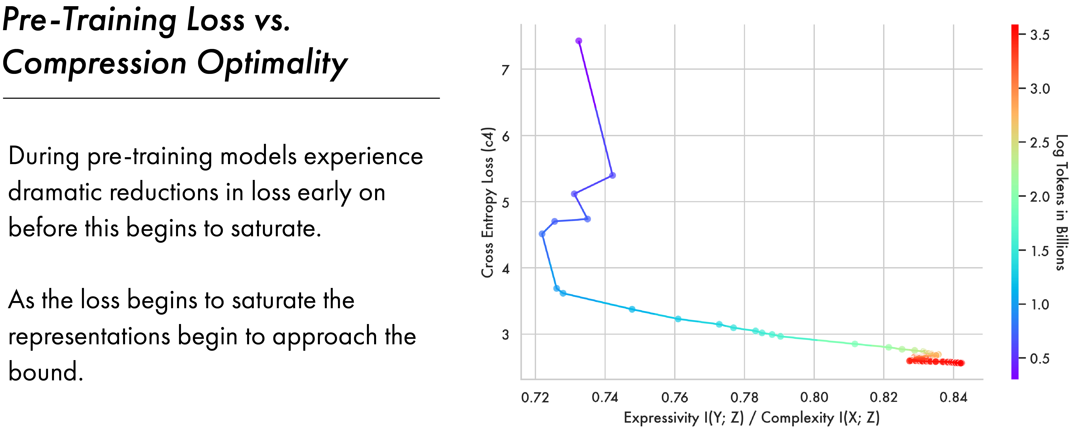
We compute the cross-entropy loss for the OLMo2 7b model performing next token prediction on 10,000 examples from C4. C4 is a substantive component of the OLMo2 pre-training data (OLMo et al. 2025) and so gives us a proxy for in-distribution performance on the model’s training set. This follows a previously attested dynamic, where earlier steps dramatically decrease the loss before this begins to slowly saturate. The figure above shows this loss plotted against the ratio between expressivity \(I(Y;Z)\) and complexity \(I(X;Z)\). This ratio acts as a distance to the bound — as this quantity approaches 1.0 models approach the bound. The figure shows how models begin to approach the bound as the loss on C4 begins to saturate, broadly aligning with Shwartz-Ziv and Tishby (2017).
G — Estimator Robustness
Our work does not introduce the soft entropy estimator but is the first to apply it in this context. As a result we run some robustness experiments to see how the results vary under different hyper-parameters and data distributions.
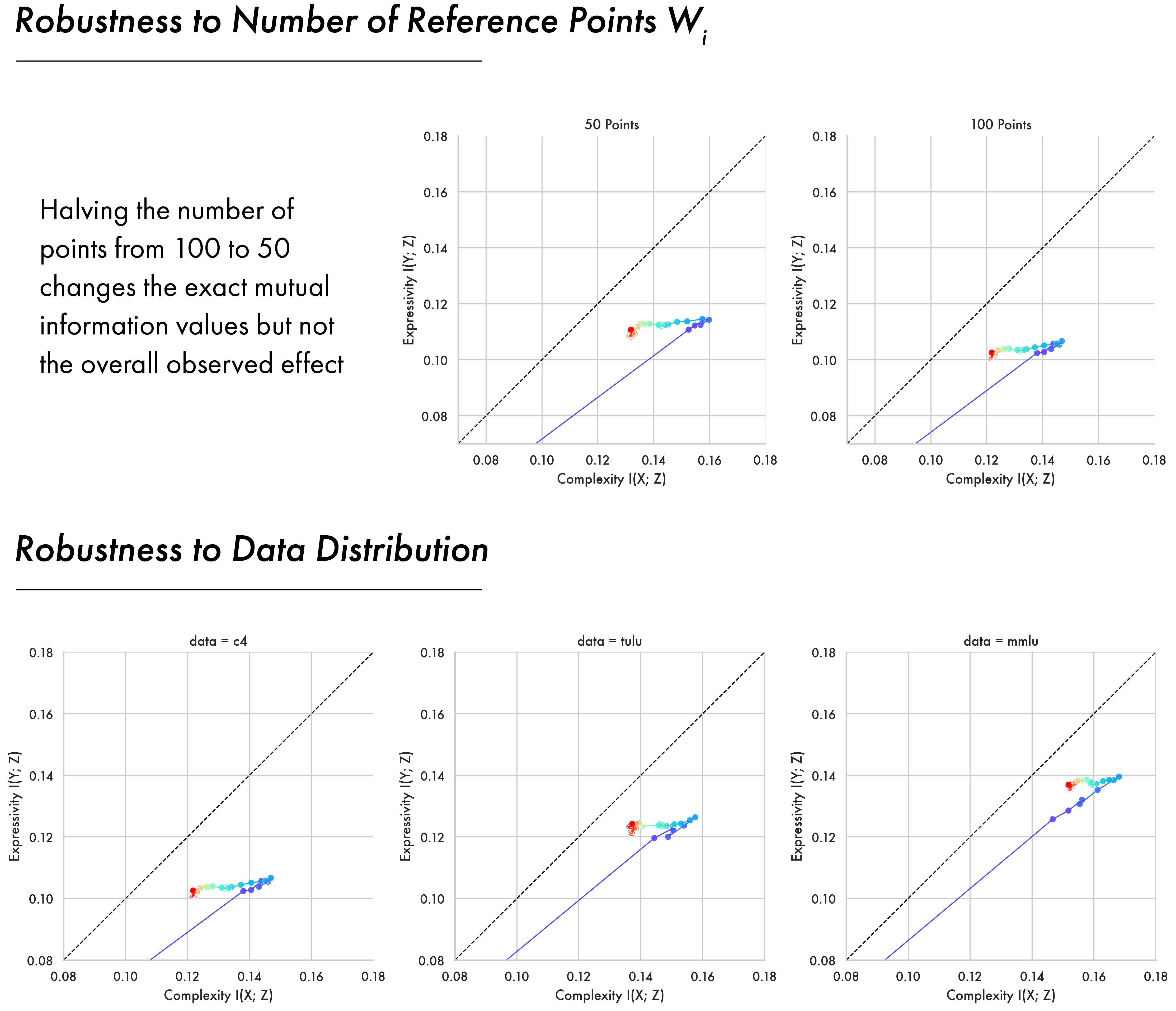
G.1 — Robustness to Data Distribution
Core results in the paper show information plane trajectories computed using C4 as this dataset forms a substantive part of the pre-training data for the OLMo2 models. To verify that the overall pattern of expansion and compression is robust across data distributions we analyse the pre-training checkpoints of the OLMo2 7B model across data from C4, Tulu (Lambert et al. 2024), and MMLU (Hendrycks et al. 2020). The two-phase pattern proves consistent across all of them with a fitting phase followed by a compression phase where models approach the bound. There are individual variations for each dataset, with Tulu and MMLU having higher mutual informations than C4. This may reflect that MMLU and Tulu are more domain-specific than C4, which is a broad crawl of the internet.
G.2 — Robustness to Number of Reference Points
The Soft Entropy estimator relies on a soft-quantisation of a model’s embedding space, whereby each representation is softly assigned to \(n\) points \(w_i\) sampled uniformly at random from the surface of the unit sphere. Experiments in the paper use \(n=100\). Here we show the core 7b model pre-training time-course computed for C4 with token backoff using \(n=100\) and \(n=50\). The results show the same overall pattern of expansion and compression with small changes to the exact mutual information values. Given this estimator resembles a differentiable relaxation of a binning-based estimate, it is relevant to note that in binning based approaches increasing the number of bins reduces mutual information by assigning similar representations to an increasing number of different bins (Paninski 2003). The results seen here are consistent with this effect — 100 points achieves slightly lower mutual information than 50 points.
G.3 — Language is a Long-Tailed Distribution: Computing Mutual Information with Means
As noted in Section 3.1, the quantity estimated here is mutual information, which uses an expectation over conditional entropies:
\[ I(X; Z) := \mathcal{H}(Z) - \sum_{x \in X} P(X=x)\, \mathcal{H}(Z| X=x) \]
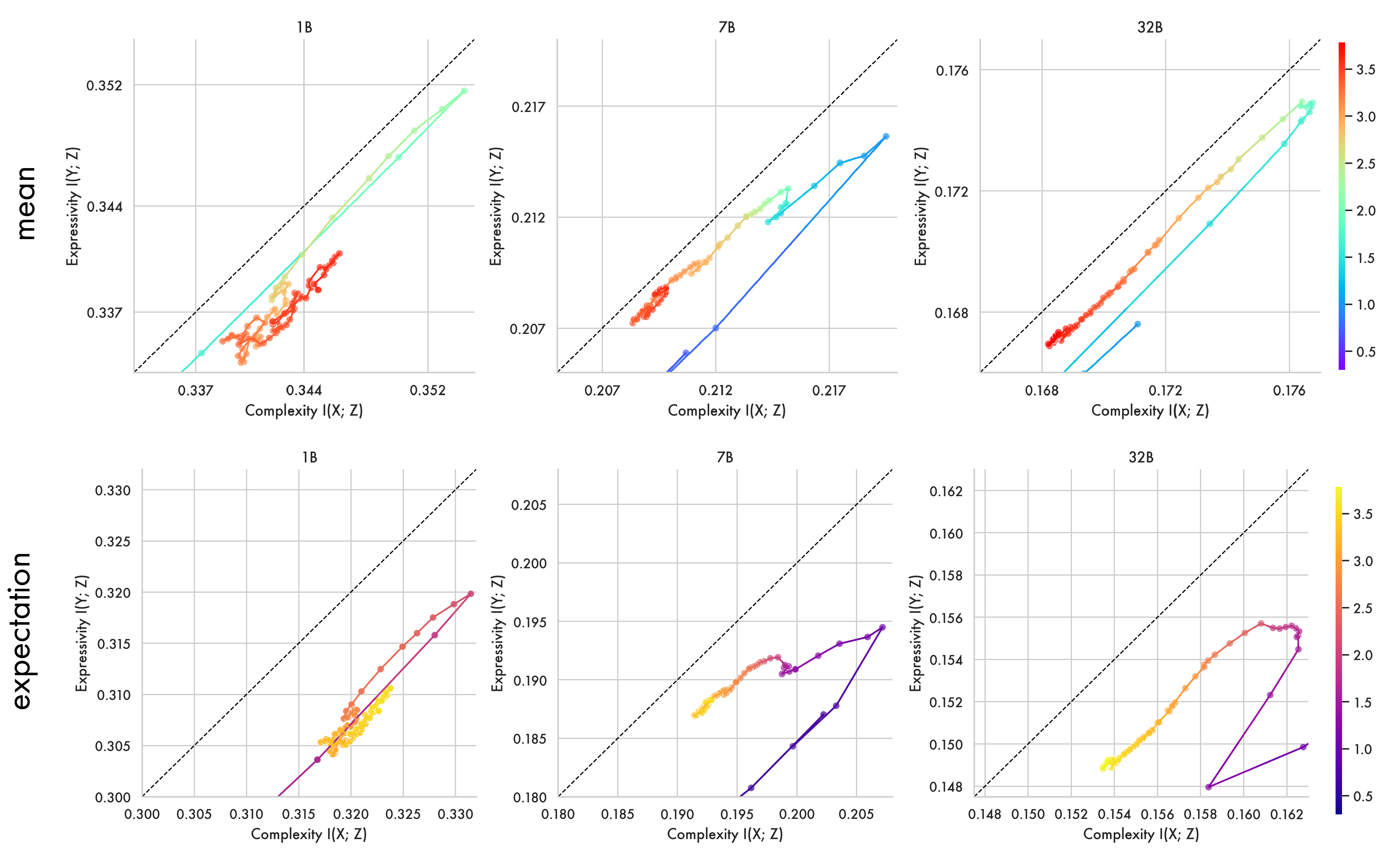
Here we recompute the core pre-training analyses for the 1B, 7B and 32B models using a mean — to see how treating each event as equiprobable affects the analysis. Given language is known to be Zipfian distributed a small number of high-probability patterns likely drive the mutual information. It is worth noting when using a mean the resulting quantity is not the true mutual information, and so the information bottleneck bound does not necessarily apply:
\[ I(X; Z) := \frac{1}{|X|}\sum_{x \in X} \mathcal{H}(Z) - \mathcal{H}(Z| X=x) \]
As shown in the figure below, estimates computed with the mean and with the expectation both show the same two-phase pattern, with models first expanding representations before compressing towards the bound. When taken as a mean the quantity reflects the mean mutual information per label — like mean mutual information per token — rather than being weighted by the exponentially distributed token representations.
H — Datasets, Models, and Compute
H.1 — Licenses for Models and Datasets
As noted in Section 3, we use two datasets for estimation — Tulu (Lambert et al. 2024) and C4 (Raffel et al. 2020), both of which fall under the Open Data Commons Attribution License (ODC-By) v1.0. We also use MMLU Pro for behavioural evaluation (Wang et al. 2024), which falls under the Apache License (Version 2.0).
We study a wide array of models; license information grouped by model family:
- OLMo: The code and models are released under Apache 2.0.
- Gemma: Released under the Gemma license: https://ai.google.dev/gemma/terms
- Llama: Released under the Llama license: https://www.llama.com/llama3/license/
- Qwen: The code and models are released under Apache 2.0.
- Aya/Command: Released under the Creative Commons Attribution Non Commercial 4.0.
- Pythia: The code and models are released under Apache 2.0.
H.2 — Compute Resource and Complexity
The estimation procedure used here has low complexity for an entropy estimator, requiring only a dot-product and softmax. The majority of compute expense comes from the model’s forward pass required to compute the estimate. The complexity of this depends on the size of the model. In experiments here estimates required encoding 10,000 samples from C4 and Tulu. This process takes approximately 10, 40, or 70 minutes on 2, 4, or 8 H100 GPUs respectively (number required depending on model size). Given this we estimate the total number of GPU hours required for the results in this paper at approximately 3,600 H100 hours.
I — Acknowledgements, Ethics & Reproducibility
I.1 — Acknowledgements
We would like to thank Kenny Smith for his role in developing the core ideas presented here in earlier versions of this project.
I.2 — Ethics Statement
All experiments reported here use publicly available datasets and pretrained models obtained under their original licenses; see Appendix H.1 for details. To our knowledge, these datasets contain no personally identifiable information, and we are in compliance with their terms of use. No additional data were collected. More generally, all authors have read and adhered to the ICLR Code of Ethics. To the best of our knowledge, these results and their dissemination do not raise any ethical concerns.
I.3 — Reproducibility Statement
All datasets and pre-trained models used in our experiments are publicly available (see Appendix H.1). All code has been released at https://github.com/hcoxec/soft_h. Appendix H.2 contains details of compute resources necessary to reproduce these findings.